Gaussian
Gaussian is one of the most widely used and well-known quantum chemistry software packages for studying the electronic structure, energetic properties, and spectroscopic characteristics of molecules.
The program supports a variety of quantum chemical methods, including Hartree-Fock (HF), Density Functional Theory (DFT), and post-Hartree-Fock approaches.
The development of Gaussian began in the 1970s under the leadership of John A. Pople and his collaborators. The software package played a major role in the advancement of computational molecular modeling, and the theoretical developments associated with it contributed to John A. Pople being awarded the 1998 Nobel Prize in Chemistry.
Main Applications of Gaussian
The program can be applied to a wide range of computational tasks, including:
molecular geometry optimization
determination of electron densities and molecular orbitals
investigation of reaction mechanisms
transition-state searches
calculation of reaction and activation energies
prediction of vibrational frequencies and infrared spectra
calculation of NMR, UV-Vis, and other spectroscopic parameters
modeling solvent effects
Gaussian calculations make it possible to investigate molecular systems that are difficult or impossible to study experimentally.
Structure of a Gaussian Input File
Gaussian calculations are initiated using text-based input files. A typical input file consists of five main sections:
resource specifications
route section
title
charge and multiplicity
molecular geometry
A simple example for the geometry optimization of a water molecule:
%Mem=4GB
%NProcShared=8
%Chk=water.chk

#P B3LYP/def2SVP Opt

Water geometry optimization

0 1
O      0.000000      0.000000      0.000000
H      0.758602      0.000000      0.504284
H     -0.758602      0.000000      0.504284
Note
It is recommended to leave four or five blank lines after the molecular geometry at the end of the input file to avoid potential issues when Gaussian reads the file.
Resource Specifications
Lines beginning with the % character define the computational resources
available for the calculation.
%Mem=4GB
%NProcShared=8
%Chk=water.chk
%Mem: amount of memory available to the calculation%NProcShared: number of processor cores available for parallel execution%Chk: name of the checkpoint file
The checkpoint file stores the wavefunction and other information that can be reused in subsequent calculations.
Route Section
The route section defines the type of calculation to be performed.
#P B3LYP/def2SVP Opt
In this example:
B3LYPis the selected density functionaldef2-SVPis the basis setOptrequests a geometry optimizationPproduces more detailed output
Multiple tasks can be requested simultaneously:
#P B3LYP/def2TZVP Opt Freq
This input performs a frequency calculation after the geometry optimization has been completed.
Running Gaussian Calculations
On Linux systems, calculations are typically launched from the command line.
g16 < water.gjf > water.log
The results of the calculation are written to the .log file, while
intermediate information is stored in the checkpoint file.
For calculations with long execution times, it is often convenient to run
Gaussian independently of the terminal session. A simple solution is to use
the nohup command, which ensures that the process continues running even
after the terminal has been closed.
nohup g16 < water.gjf > water.log &
The components of the command are:
nohup: detaches the process from the terminalg16: launches Gaussian 16< water.gjf: redirects the input file> water.log: saves the output to the log file&: executes the calculation in the background
After the command is issued, the shell prompt returns immediately while the calculation continues to run in the background.
Example 1: Geometry Optimization of a Water Molecule
The goal of geometry optimization is to determine the most stable structure of a molecule, i.e., to find the geometry corresponding to the minimum potential energy of the system. During the optimization process, Gaussian iteratively modifies the atomic coordinates until the specified convergence criteria are satisfied.
The following example demonstrates the geometry optimization of a water molecule (H₂O) using the B3LYP functional and the def2-SVP basis set.
Contents of the input file
water_opt.gjf:
%chk=job.chk
%nprocshared=10
%mem=40GB
#P B3LYP/def2SVP Opt

H2O Optimization

0 1
O    0.000000    0.200000    0.000000
H    1.200000    0.000000    0.000000
H   -1.200000    0.000000    0.000000
In the input file:
%chk=job.chkcreates the checkpoint file used to store data generated during the optimization;%nprocshared=10allows the use of ten processor cores;%mem=40GBallocates 40 GB of memory;#P B3LYP/def2SVP Optspecifies the quantum chemical method and requests a geometry optimization;0 1defines the molecular charge (0) and multiplicity (1, singlet state).
The calculation can be started with the following command:
nohup g16 < water_opt.gjf > water_opt.log &
Files Generated During the Calculation
After the Gaussian calculation has finished, several files are generated in the
working directory. The most important are the log file
(water_opt.log) and the
checkpoint file (job.chk).
The log file (
.log) contains:the contents of the input file,
the computational method and basis sets used,
the results of the SCF cycles,
the optimization steps,
the energies of individual cycles,
changes in geometric parameters,
the optimized coordinates,
the final status of the calculation.
The checkpoint file (
.chk) is a binary file that contains, among other things:the optimized geometry,
the molecular orbitals,
the electron density,
the wavefunction,
various intermediate computational data.
How Can You Tell Whether the Calculation Finished Successfully?
In the case of a successful calculation, the following line appears in the output:
Optimization completed.
followed by the message near the very end of the file:
Normal termination of Gaussian 16.
This is the most important message. If it does not appear at the end of the output, the calculation either terminated due to an error or is still running.
Checking Optimization Convergence
During the optimization, Gaussian evaluates the convergence criteria after every cycle. A block similar to the following can be found in the log file:
        Item               Value     Threshold  Converged?
Maximum Force            0.000318     0.000450     YES
RMS     Force            0.000268     0.000300     YES
Maximum Displacement     0.001846     0.001800     NO
RMS     Displacement     0.001605     0.001200     NO
The optimization is considered successful only when all criteria are marked
with YES.
Where Is the Optimized Geometry Located?
The optimized coordinates can be found immediately after the
Optimization completed.
message.
In the log file, search for the following text:
Standard orientation:
The last occurrence of this block contains the final optimized geometry. In our case:
                         Standard orientation:
---------------------------------------------------------------------
Center     Atomic      Atomic             Coordinates (Angstroms)
Number     Number       Type             X           Y           Z
---------------------------------------------------------------------
  1          8           0       -0.000000   -0.000000    0.120246
  2          1           0       -0.000000    0.756742   -0.480983
  3          1           0       -0.000000   -0.756742   -0.480983
---------------------------------------------------------------------
The final Standard orientation block always contains the current optimized
geometry.

Location of the Optimized Energy
The most important result of a geometry optimization is the total electronic energy. This value appears at the end of the SCF cycles:
SCF Done: E(RB3LYP) = -76.3583156379
The energy of the optimized structure can be obtained from the SCF Done
line in the final optimization cycle.
Example 2 - Frequency Calculation and Thermochemistry of Ethanol
Following geometry optimization, one of the most important steps in quantum chemical calculations is the frequency calculation. On the one hand, it verifies that the optimized structure corresponds to a true minimum on the potential energy surface; on the other hand, it enables the determination of various thermochemical properties.
During a frequency calculation, Gaussian computes the harmonic vibrational frequencies of the molecule and derives quantities such as the zero-point energy, entropy, and Gibbs free energy.
Input File
In the simplest case, a frequency calculation can be performed on a previously optimized structure.
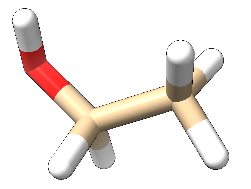
Assume that an optimized structure is available
(ethanol_opt.xyz), which can be
used to prepare the frequency calculation input file
(ethanol_freq.gjf):
%chk=job.chk
%nprocshared=10
%mem=40GB
#P B3LYP/def2SVP Freq

Ethanol Frequency Calculation

0 1
H          -2.08221584675915      0.44154569995427      0.06677273956542
C          -1.21103849015378     -0.23021760296498     -0.01038523298038
H          -1.27931552008987     -0.95748995777425      0.81806656011703
C           0.09701554266621      0.55117522315977      0.05144703042052
O           1.23811100304160     -0.26504753081186     -0.11984319301300
H           0.14696459615673      1.12741911770514      0.99961233843453
H           1.25806639502500     -0.90617726301460      0.60317183521497
H           0.12997269251367      1.29210920605380     -0.76479381040057
H          -1.28320146410041     -0.78854025890729     -0.95745612375851
Running the Calculation
nohup g16 < ethanol_freq.gjf > ethanol_freq.log &
During execution, the log file
ethanol_freq.log is
generated.
Objectives of the Calculation
The frequency calculation provides answers to several important questions.
1. Verification of a True Minimum
For a true minimum, all vibrational frequencies must be positive.
                     1                      2                      3
                     A                      A                      A
Frequencies --    279.5697               320.8435               426.2556
If a negative (imaginary) frequency appears, the structure does not correspond to a true minimum but rather to a transition state or an improperly converged geometry.
Interpretation:
0 imaginary frequencies → minimum structure
1 imaginary frequency → transition state
2 or more imaginary frequencies → unconverged or incorrect structure
2. Calculation of the IR Spectrum
Gaussian computes the infrared intensity for each vibrational mode.
Frequencies --    279.5697               320.8435               426.2556
IR Inten    --      5.4936               110.0845                21.4718
These data can be used directly to generate a theoretical infrared spectrum.
Thermochemical Data
One of the most important outcomes of a frequency calculation is the evaluation of thermochemical corrections. Near the end of the log file, the following block can be found:
Zero-point correction=                           0.079691 (Hartree/Particle)
Thermal correction to Energy=                    0.083908
Thermal correction to Enthalpy=                  0.084852
Thermal correction to Gibbs Free Energy=         0.054379
Sum of electronic and zero-point Energies=           -154.844060
Sum of electronic and thermal Energies=              -154.839843
Sum of electronic and thermal Enthalpies=            -154.838899
Sum of electronic and thermal Free Energies=         -154.869372
Molecules are not completely motionless even at absolute zero temperature.
Due to quantum-mechanical effects, they possess zero-point energy. This is
represented by the value given under Zero-point correction.
In Gaussian, thermal corrections are reported by default at a temperature of 298.15 K and a pressure of 1 atm.
The following corrections are provided:
Thermal correction to Energy
Thermal correction to Enthalpy
Thermal correction to Gibbs Free Energy
These values are used to calculate reaction enthalpies and Gibbs free energies of reaction.
The lines beginning with Sum of electronic and ... contain the quantities
most commonly used for:
reaction energy calculations,
determination of reaction enthalpies,
investigation of equilibrium processes,
comparison of conformational stability.
Visualization of Vibrational Modes
Vibrational modes can be visualized using either GaussView or ChimeraX.
The normal modes associated with the calculated frequencies can be used to:
identify possible imaginary frequencies,
determine the character of a transition state,
interpret experimental IR spectra.
Example 3: UV-Vis Spectrum Calculation of Caffeine Using TD-DFT
After completing geometry optimization and frequency calculations, a common task is the investigation of the electronic excited states of molecules. For this purpose, Gaussian provides the Time-Dependent Density Functional Theory (TD-DFT) method, which makes it possible to determine the energies, wavelengths, and intensities of electronic transitions.
In this example, we demonstrate the calculation of the UV-Vis spectrum of caffeine.
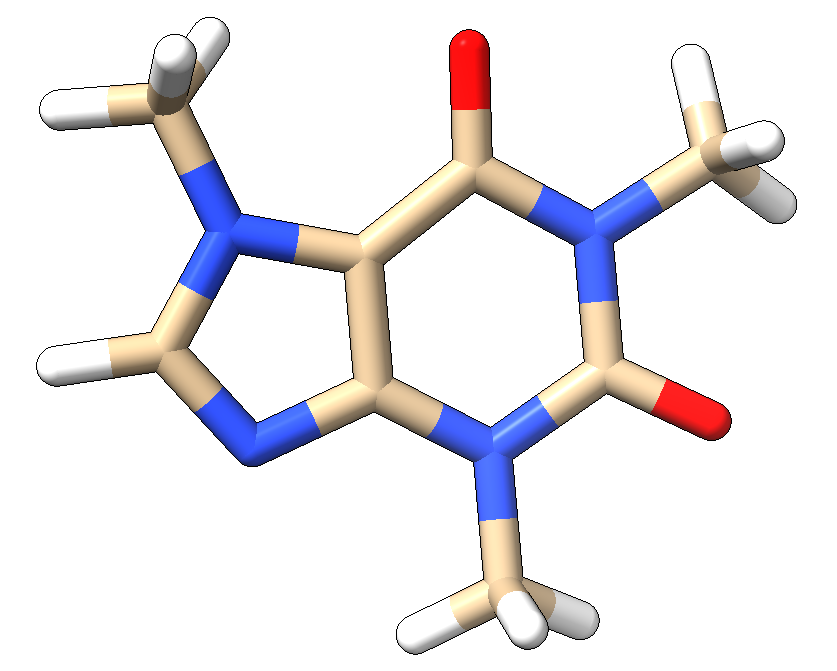
Purpose of the Calculation
A TD-DFT calculation can be used to determine:
the energies of the first few excited states,
the absorption wavelengths,
the oscillator strengths,
the nature of the electronic transitions,
the data required for simulating a UV-Vis spectrum.
In the case of caffeine, the objective is to identify which electronic transitions are responsible for the absorption bands observed in the ultraviolet region.
TD-DFT Calculation
Let us assume that the caffeine.chk file obtained during the geometry
optimization is available. To determine the excited states, for example, the
first 20 electronic transitions can be calculated.
%chk=caffeine.chk
%nprocshared=25
%mem=100GB
#P TD(NStates=20) B3LYP/def2TZVP Geom=AllCheck Guess=Read

Caffeine UV-Vis calculation
The most important keywords in the input file
(caffeine_uvvis.gjf)
are:
TD: starts a TD-DFT calculation;NStates=20: calculates the first 20 excited states;Geom=AllCheck: reads the molecular geometry from the checkpoint file;Guess=Read: reads the previously calculated wavefunction;B3LYP/def2TZVP: specifies the functional and basis set used.
Note
This approach is generally faster and more reliable than specifying the molecular coordinates again in the input file.
Running the Calculation
nohup g16 < caffeine_uvvis.gjf > caffeine_uvvis.log &
The calculation generates the files
caffeine_uvvis.log and
caffeine.chk.
The log file contains:
the energies of the excited states,
the absorption wavelengths,
the oscillator strengths,
the molecular orbitals involved in the electronic transitions.
Results of the Excited-State Calculations
The most important results can be found in the log file in the following form:
    Excitation energies and oscillator strengths:

Excited State   1:      Singlet-A      4.6489 eV  266.69 nm  f=0.1302  <S**2>=0.000
     51 -> 52         0.68850
This state for optimization and/or second-order correction.
Total Energy, E(TD-HF/TD-DFT) =  -680.469471377
Copying the excited state density for this state as the 1-particle RhoCI density.

Excited State   2:      Singlet-A      4.9654 eV  249.70 nm  f=0.0000  <S**2>=0.000
     47 -> 52         0.16787
     50 -> 52         0.67236

Excited State   3:      Singlet-A      5.6494 eV  219.46 nm  f=0.0203  <S**2>=0.000
     48 -> 52         0.19048
     49 -> 52         0.52954
     51 -> 53         0.30801
     51 -> 54        -0.27680

   ...
The meaning of the individual quantities is:
eV: transition energynm: absorption wavelengthf: oscillator strength
The intensity of an absorption band is characterized by its oscillator strength. In a UV-Vis spectrum, transitions with higher oscillator strengths generally appear as the dominant absorption bands.
For each excited state, Gaussian reports the molecular orbitals involved in the corresponding electronic transition. For example:
Excited State   1:      Singlet-A      4.6489 eV  266.69 nm  f=0.1302  <S**2>=0.000
 51 -> 52         0.68850
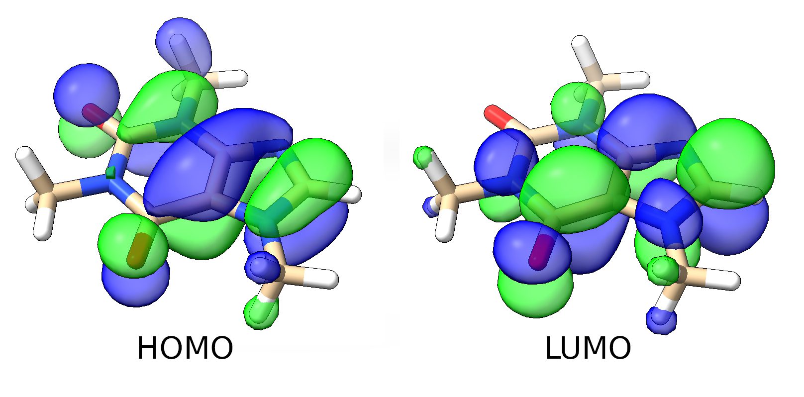
This indicates that the first excited state is primarily composed of the 51→52 molecular orbital transition. In this particular case, it corresponds to a HOMO→LUMO-type excitation.
Generation of the UV-Vis Spectrum
To construct a UV-Vis spectrum, the excitation wavelengths and their corresponding oscillator strengths are required. These values can be extracted directly from the TD-DFT output.
Transition |
Wavelength (nm) |
f |
|---|---|---|
1 |
266.69 |
0.1302 |
2 |
249.70 |
0.0000 |
3 |
219.46 |
0.0203 |
4 |
207.27 |
0.1314 |
5 |
206.78 |
0.0002 |
6 |
203.21 |
0.0057 |
7 |
201.75 |
0.0457 |
8 |
201.19 |
0.0000 |
9 |
198.38 |
0.0000 |
10 |
196.58 |
0.3806 |
A simulated UV-Vis spectrum can be generated from the oscillator strengths by applying Gaussian broadening functions to the individual transitions.
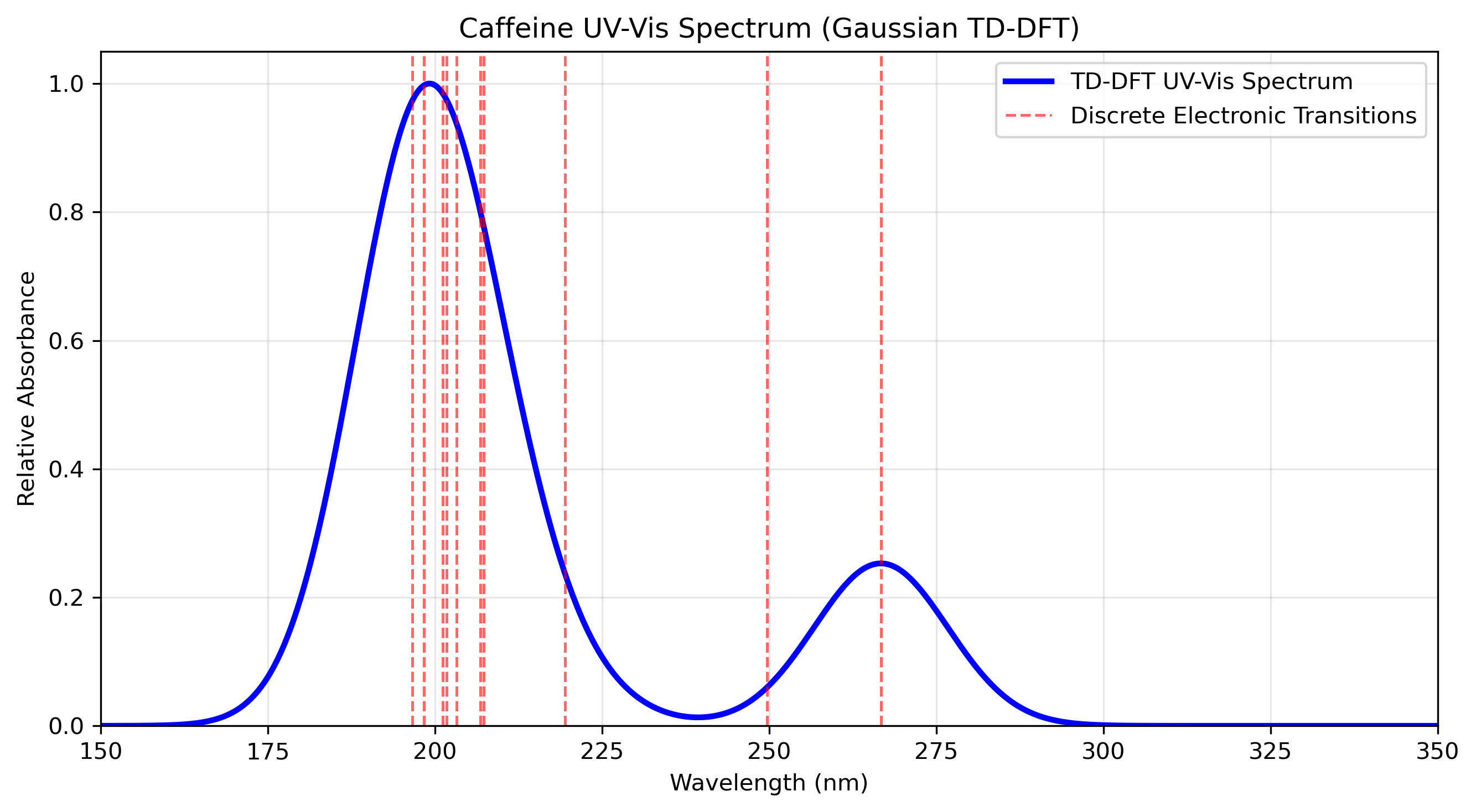
Python script used to generate the spectrum:
Visualizing Molecular Orbitals with ChimeraX
ChimeraX is capable of displaying molecular orbitals. However, the generated
caffeine.chk file must first be converted into a formatted checkpoint file:
formchk caffeine.chk caffeine.fchk
The resulting
caffeine.fchk
file can then be opened directly in ChimeraX. To visualize individual molecular
orbitals, use the following tool:
Tools → Quantum Chemistry → Orbital Viewer
Example 4: NMR Chemical Shift Calculation for Methane
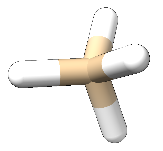
One of the spectroscopic calculations frequently performed with Gaussian is the determination of NMR chemical shifts. Gaussian uses the GIAO (Gauge-Independent Atomic Orbital) method to calculate magnetic shielding tensors, from which chemical shifts can be derived. In this example, we demonstrate the calculation of the ¹H and ¹³C NMR properties of a simple methane molecule (CH₄).
Purpose of the Calculation
An NMR calculation can be used to determine:
isotropic magnetic shielding constants (σ),
chemical shifts (δ),
characteristics of the local environments of different nuclei,
data required for the interpretation of experimental NMR spectra.
For direct comparison of chemical shifts, a reference compound is usually required. For organic compounds, the most commonly used reference is tetramethylsilane (TMS).
NMR Calculation
Let us assume that the methane.chk file generated during geometry
optimization is available. The optimized structure stored in this file can be
used to determine the NMR shielding constants.
Input file
(methane_nmr.gjf):
%chk=methane.chk
%nprocshared=25
%mem=100GB
#P B3LYP/def2TZVP NMR=GIAO Geom=AllCheck Guess=Read

Methane NMR Calculation
Important keywords:
NMR=GIAO: requests the use of the GIAO method;Geom=AllCheck: reads the molecular geometry from the checkpoint file;Guess=Read: uses the previously calculated wavefunction;B3LYP/def2TZVP: specifies the functional and basis set used.
Starting the Calculation
nohup g16 < methane_nmr.gjf > methane_nmr.log &
During the calculation, the log file
methane_nmr.log
is generated.
Location of the Results
The magnetic shielding data can be found in the following section of the log file:
SCF GIAO Magnetic shielding tensor (ppm):
For each atom, the block contains the shielding tensor and its isotropic average.
1  H    Isotropic =    31.7133   Anisotropy =     8.8693
2  C    Isotropic =   190.3591   Anisotropy =     0.0020
3  H    Isotropic =    31.7133   Anisotropy =     8.8693
4  H    Isotropic =    31.7132   Anisotropy =     8.8692
5  H    Isotropic =    31.7133   Anisotropy =     8.8693
Since methane has tetrahedral symmetry, all four hydrogen atoms are completely equivalent and therefore have identical shielding values.
Determination of Chemical Shifts
Gaussian directly calculates shielding constants, denoted by σ.
Chemical shifts are calculated relative to a reference compound:
where
\(\delta\) is the chemical shift,
\(\sigma_{ref}\) is the shielding constant of the reference compound,
\(\sigma_{sample}\) is the shielding constant of the atom under investigation.
Consequently, accurate chemical shifts require a TMS calculation performed using the same computational method and basis set as the molecule of interest.
Example 5: Transition State Search for an SN2 Reaction
In addition to geometry optimizations, frequency calculations, and spectroscopic studies, one of the most important applications of Gaussian is the investigation of reaction mechanisms. In such calculations, it is possible to determine the highest-energy point along the reaction pathway, known as the transition state (TS).
As an example, we consider the classical SN2 reaction:
The SN2 reaction proceeds in a single elementary step. In the transition state, the carbon atom is simultaneously partially bonded to both the chlorine and bromine atoms.
A transition-state search can provide:
the geometry of the transition state,
the activation energy,
the reaction coordinate,
the imaginary frequency,
the connection between reactants and products.
Transition-State Structure
In the transition state of the SN2 reaction, the nucleophile and the leaving group are located at approximately equal distances from the carbon atom.
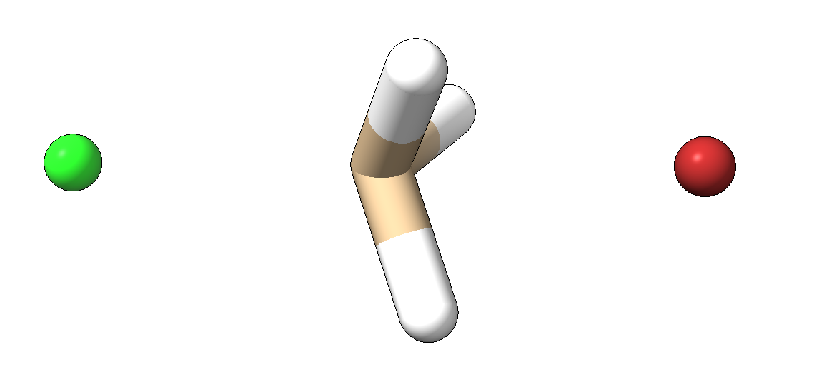
The system exhibits an approximately trigonal-bipyramidal geometry.
Transition-State Optimization
The input file used
(sn2_tsopt.gjf)
is shown below:
%chk=sn2_ts.chk
%nprocshared=25
%mem=100GB

#P B3LYP/def2TZVP Opt=(TS,CalcFC,NoEigenTest)

SN2 transition state search

-1 1
H         -1.91051       -1.20940        0.64919
H         -1.91051       -0.61336       -0.99331
H         -1.91051        0.51106        0.34413
C         -1.55384       -0.43723        0.00000
Cl        +0.64616       -0.43723        0.00000
Br        -3.75384       -0.43723        0.00000
The keywords have the following meanings:
TS: requests a transition-state search;CalcFC: calculates the initial Hessian matrix;NoEigenTest: applies a more relaxed convergence treatment in problematic cases.
Transition-state optimization is generally much more sensitive to the quality of the starting geometry than a standard geometry optimization.
Running the Calculation
nohup g16 < sn2_tsopt.gjf > sn2_tsopt.log &
During the calculation, the log file
sn2_tsopt.log
is generated.
Frequency Calculation on the Transition State
To verify that the optimized structure is indeed a transition state, a
frequency calculation must be performed. The corresponding input file
(sn2_ts_freq.gjf) is:
%chk=sn2_ts.chk
%nprocshared=25
%mem=100GB

#P B3LYP/def2TZVP Freq Geom=AllCheck Guess=Read

SN2 TS frequency calculation
Execution:
nohup g16 < sn2_ts_freq.gjf > sn2_ts_freq.log &
The calculation generates the log file
sn2_ts_freq.log.
For a true transition state, exactly one imaginary frequency must be present. In this example:
                     1                      2                      3
                     A                      A                      A
Frequencies --   -304.5943               170.3495               173.0307
Thus, the imaginary frequency corresponding to the reaction coordinate is -304.6 cm⁻¹.
Interpretation:
Number of Imaginary Frequencies | Meaning |
|
|---|---|
0 |
Minimum |
1 |
Transition State |
>1 |
Incorrect TS |
Visualization of the Vibrational Mode
One of the most important steps in validating a transition state is to animate the vibrational mode associated with the imaginary frequency.
ChimeraX can open the sn2_ts_freq.log file. The vibrational mode
corresponding to the imaginary frequency can then be visualized using:
Tools → Quantum Chemistry → Visualize Normal Modes
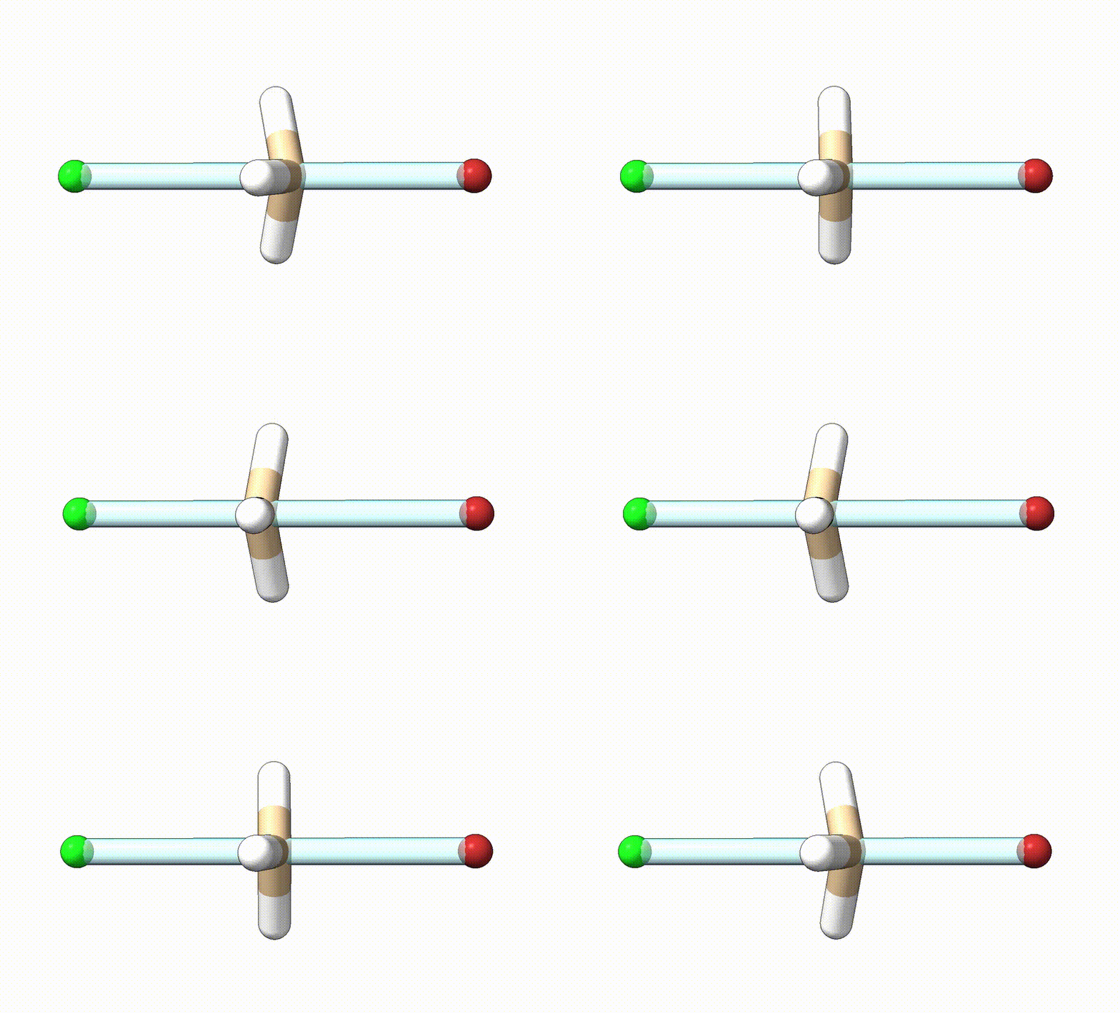
The animated mode should show motion along the reaction coordinate, i.e., the simultaneous breaking of the C-Br bond and formation of the C-Cl bond.
Determination of the Activation Energy
The activation energy can be calculated from the difference between the energy of the reactants and that of the transition state:
where
\(E_{\mathrm{a}}\) is the activation energy,
\(E_{\mathrm{TS}}\) is the energy of the transition state,
\(E_{\mathrm{reactant}}\) is the energy of the reactant state.
The activation energy represents the energy barrier that must be overcome for the reaction to proceed and is one of the key parameters governing reaction kinetics.
Example 6: Accounting for Solvent Effects Using the SMD Model
A significant fraction of quantum chemical calculations are not concerned with gas-phase systems, but rather with processes occurring in solution. The presence of a solvent can substantially influence the stability, molecular geometry, reaction energies, and spectroscopic properties of molecules.
Gaussian supports a variety of implicit solvent models. One of the most commonly used among them is the SMD (Solvation Model based on Density) model.
In this example, we compare the energy and structure of the caffeine molecule in the gas phase and in aqueous solution. The presence of the solvent can affect:
the total energy,
the HOMO-LUMO gap,
the UV-Vis spectrum,
the dipole moment,
the NMR chemical shifts.
In this documentation, we focus on the first three properties.
Geometry Optimization in Aqueous Solution
In Section Példa 4 - NMR kémiai eltolódások számítása metánon, the caffeine molecule was previously optimized in the gas phase, and its UV-Vis spectrum was calculated based on the first ten electronic excitations.
To activate the SMD solvent model, the SCRF keyword must be used. The input
file (caffeine_water_opt.gjf)
is shown below:
%chk=caffeine_water.chk
%nprocshared=25
%mem=100GB

#P B3LYP/def2TZVP Opt SCRF=(SMD,Solvent=Water)

Caffeine in water

0 1
N      1.5808      0.7027     -0.2279
C      1.7062     -0.7374     -0.2126
N      0.5340     -1.5671     -0.3503
C      0.3231      1.3600      0.0274
C     -0.8123      0.4553      0.0817
C     -0.6967     -0.9322     -0.0662
N     -2.1886      0.6990      0.2783
C     -2.8512     -0.5205      0.2532
N     -1.9537     -1.5188      0.0426
C      0.6568     -3.0274     -0.1675
O      2.8136     -1.2558     -0.1693
O      0.2849      2.5744      0.1591
C     -2.8096      2.0031      0.5032
C      2.8301      1.5004     -0.1968
H     -3.9271     -0.6787      0.3762
H      1.4823     -3.4046     -0.7865
H     -0.2708     -3.5204     -0.4868
H      0.8567     -3.2990      0.8788
H     -2.4123      2.7478     -0.2017
H     -2.6042      2.3621      1.5221
H     -3.8973      1.9344      0.3695
H      3.5959      1.0333     -0.8314
H      3.2249      1.5791      0.8255
H      2.6431      2.5130     -0.5793
Important keywords:
SCRF: activates the solvent model;Water: specifies water as the solvent.
Running the Calculation
nohup g16 < caffeine_water_opt.gjf > caffeine_water_opt.log &
During the calculation, the log file
caffeine_water_opt.log
is generated.
Solvation Energy
The results of the gas-phase and solution-phase calculations can be compared:
System |
Energy (Hartree) |
|---|---|
Gas phase |
-680.640316438 |
Water |
-680.659984870 |
The difference between the two energies provides an estimate of the stabilizing effect of solvation.
UV-Vis Spectrum in Solution
The TD-DFT example presented earlier can be readily extended to aqueous solution by including the keyword:
SCRF=(SMD,Solvent=Water)
in the input file
(caffeine_water_uvvis.gjf).

The calculated results show that the discrete electronic transitions shift toward shorter wavelengths in the presence of the solvent.
HOMO-LUMO Energy Gaps
System |
Energy Gap |
|---|---|
Gas phase |
0.18744 Hartree |
Water |
0.18908 Hartree |
The slight increase in the HOMO-LUMO energy gap indicates that the solvent stabilizes the occupied and virtual molecular orbitals to different extents, thereby modifying the electronic structure of the molecule.