MOPAC
MOPAC is a semi-empirical quantum mechanical software package used for investigating the electronic structure, geometry, and various properties of molecules and materials. The program operates based on an input file and saves the results of the calculation in several different output files.
The most common applications of MOPAC include single-point energy calculations, geometry optimizations, vibrational frequency calculations, and the inclusion of solvent effects through implicit solvent models.
To run a MOPAC calculation, a text-based input file must be created containing keywords, descriptive lines, and the geometry of the system under investigation. The general form of a MOPAC calculation is:
mopac example.mop
If the run is successful, the program typically generates an .out file and
an .arc file. The .out file contains the main calculation results and
log information, while the .arc file serves as an archival output file.
In the following sections, we present the structure of a MOPAC input file, the most common types of calculations, and the most important keywords.
Structure of a MOPAC Input File
The structure of a MOPAC input file is simple but sensitive to line placement. The first line contains the keywords, followed by two descriptive or comment lines, after which the molecular geometry is specified.
The general structure of a simple MOPAC input file is:
keywords
first comment or title line
second comment or description line
coordinates of atom 1
coordinates of atom 2
...
coordinates of the last atom
The geometry can be specified using Cartesian coordinates, for example by
providing the element symbol together with the x, y, and z
coordinates. MOPAC uses the name of the input file as the base name for the
generated output files.
Example input file:
AM1 OPT
Geometry optimization for a formic acid molecule

C         -3.17600        0.34760        2.01330
O         -2.05280        0.75420        2.08610
H         -4.00190        0.55050        2.69320
O         -3.48090       -0.47220        0.96340
H         -3.69880       -1.05810        0.21310
Test System
To demonstrate the use of MOPAC, formic acid (HCOOH) will be used as the test system in most of the examples. Formic acid is particularly suitable for documentation purposes because it is a relatively small molecule while already containing several chemically meaningful structural features.
In the first part of the examples, a single formic acid molecule is used to demonstrate single-point energy calculations, the basics of vibrational analysis, and, when appropriate, the treatment of solvent effects. For the geometry optimization example, we use the formic acid dimer. This system consists of two formic acid molecules forming a cyclic complex stabilized by two hydrogen bonds, making it an excellent example for demonstrating the optimization of molecular assemblies held together by hydrogen-bonding interactions.
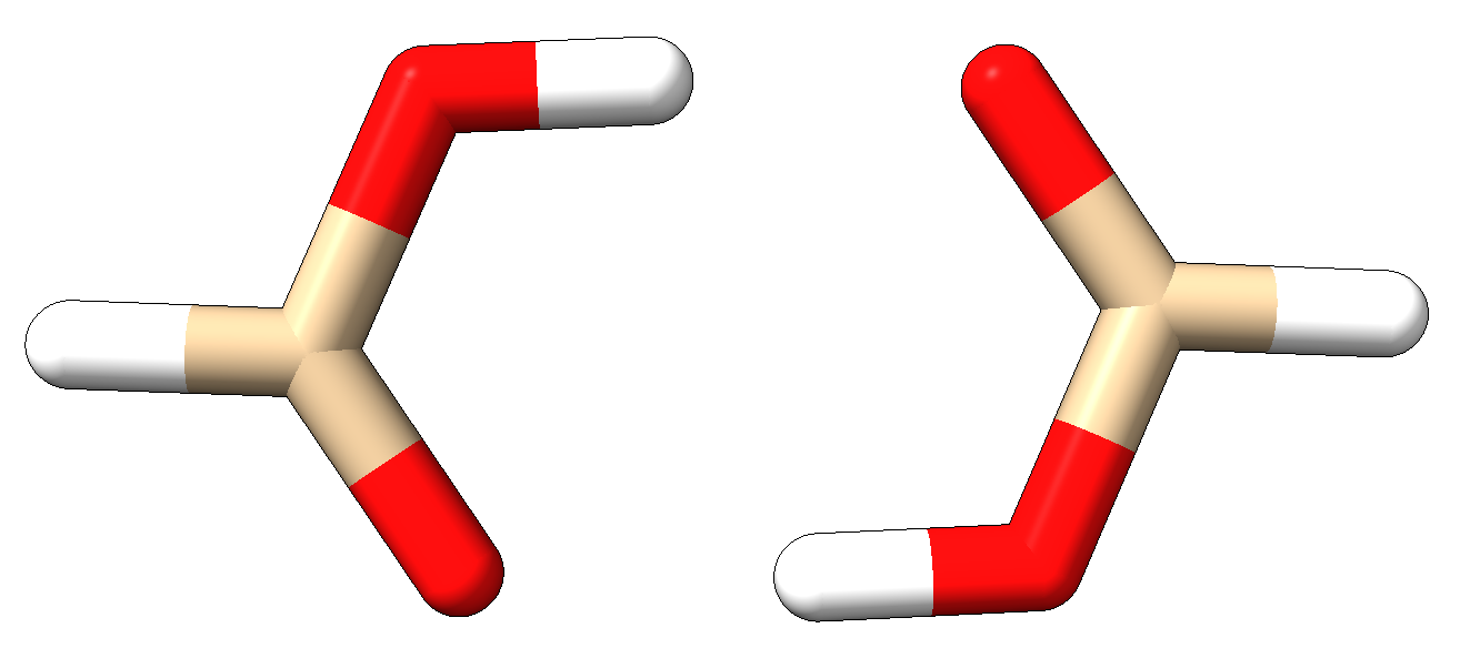
Structure of the formic acid dimer stabilized by two hydrogen bonds.
Single-Point Energy Calculation
The simplest MOPAC task is a single-point energy and electronic structure
calculation. In this type of calculation, the program performs an SCF
calculation on the supplied geometry without optimizing the molecular
structure. The 1SCF keyword can be used for single-point calculations. In
modern MOPAC versions, PM7 is a good starting point as the semi-empirical
model.
For the formic acid monomer, the following input file
formic_acid.mop can be used:
PM7 1SCF CHARGE=0
Formic acid monomer - Single-point SCF calculation

C       -3.183783941     0.327089138     2.000018081
O       -2.049843997     0.720089598     1.990180326
H       -3.984737083     0.526117507     2.708398596
O       -3.656651065    -0.494419598     1.035591555
H       -3.000638884    -0.738481355     0.338289658
In the keyword line, PM7 specifies the semi-empirical Hamiltonian,
1SCF indicates that only a single-point SCF calculation should be carried
out, and CHARGE=0 defines the system as electrically neutral.
The calculation can be started using the following command:
mopac formic_acid.mop
After the calculation has finished, it is recommended to verify that:
the calculation completed without errors;
the files
formic_acid.outandformic_acid.archave been generated;the output contains the final energy and electronic structure results.
Geometry Optimization
The purpose of geometry optimization is to determine a geometry corresponding
to a local energy minimum starting from an initial structure. By default,
MOPAC performs geometry optimization on the supplied structure, so no special
optimization keyword is required. In practice, however, the PRECISE
keyword is often used to enforce stricter convergence criteria. As a starting
point, the PM7 semi-empirical model can be employed.
The formic acid dimer is an excellent example system for geometry optimization because it is small and computationally inexpensive while already containing genuine intermolecular interactions. The two formic acid molecules form a cyclic complex stabilized by two hydrogen bonds. Consequently, the optimization demonstrates not only the relaxation of a single molecule but also the structural rearrangement of a hydrogen-bonded molecular pair. Another advantage of this system is that the optimized structure can be characterized by easily interpretable geometric parameters such as the intermolecular O···H distance.
The following input file
formic_acid_dimer_opt.mop
provides one possible starting geometry for the formic acid dimer using
Cartesian coordinates:
PM7 PRECISE
Geometry optimization for a formic acid dimer molecule

C         -0.18920       -0.20380       -0.31100
O         -1.30550       -0.63340       -0.41060
H          0.66700       -0.32750       -0.97010
O          0.18250        0.56500        0.73750
H         -0.52950        0.73710        1.40050
C         -3.18380        0.32710        2.00000
O         -2.04980        0.72010        1.99020
H         -3.98470        0.52610        2.70840
O         -3.65670       -0.49440        1.03560
H         -3.00060       -0.73850        0.33830
The coordinates above represent an example geometry of the formic acid dimer and are suitable as a starting structure for MOPAC optimization.
The calculation can be started with:
mopac formic_acid_dimer_opt.mop
The most important indicators of a successful optimization are:
the calculation finishes without errors and generates the files
formic_acid_dimer_opt.outandformic_acid_dimer_opt.arc;the output contains the line
GEOMETRY OPTIMISED USING EIGENVECTOR FOLLOWING (EF).
indicating that the geometry optimization has converged;
the output contains the text
SCF FIELD WAS ACHIEVED
indicating that the self-consistent field calculation has also converged;
the optimization progress can be followed through the
CYCLE:,GRAD.:, andHEAT:entries appearing during the optimization.
To assess the optimization process, special attention should be paid to the
HEAT: and GRAD.: values reported at each cycle. In a well-behaved
optimization, the gradient gradually decreases, while the changes in the
HEAT: value become progressively smaller as the calculation proceeds. This
indicates that the structure is approaching a minimum and the energy is
converging. The HEAT: value does not necessarily need to decrease
monotonically at every single step, but the overall trend should move toward a
stable minimum.
If the messages indicating successful geometry optimization and SCF convergence do not appear in the output, or if the gradient does not decrease below the convergence threshold, the optimization cannot be considered fully successful, even if the program generates the output files. In such cases, it is advisable to inspect the starting geometry, the selected keywords, and the SCF convergence behavior separately.
The formic acid dimer optimization example clearly illustrates that MOPAC can be used not only for individual molecules but also for the optimization of weakly bound molecular complexes stabilized by hydrogen bonding.
Frequency Calculation
After geometry optimization, it is advisable to perform a vibrational analysis on the optimized formic acid molecule. This serves two main purposes. First, the normal modes and vibrational frequencies of the molecule can be obtained. Second, it allows verification that the optimized structure actually corresponds to a minimum on the potential energy surface. Vibrational calculations on optimized geometries are included among the official MOPAC examples and therefore represent a natural next step after geometry optimization.
The FORCE keyword can be used to perform vibrational calculations.
According to the MOPAC documentation and tutorials, this keyword is used for
the calculation of vibrational frequencies and normal modes. For a molecular
structure corresponding to an energy minimum, no imaginary frequencies are
expected in the vibrational spectrum.
Note
The frequency calculation should be performed on a previously optimized structure.
One possible input file is shown below
(formic_acid_freq.mop):
PM7 FORCE
Formic acid monomer - Frequency calculation

C       -3.183979984     0.327336994     2.000311638
O       -2.049824916     0.719660125     1.989685079
H       -3.985548873     0.526173487     2.708389320
O       -3.656497428    -0.494553996     1.035761306
H       -2.999838484    -0.737146372     0.338582397
The calculation can be started using the following command:
mopac formic_acid_freq.mop
After the calculation, it is recommended to verify that:
the calculation completed without errors;
the file
formic_acid_freq.outwas generated;the output contains the vibrational frequency results;
no imaginary frequencies appear in the calculated spectrum, since their presence would indicate that the structure corresponds to a higher-order saddle point rather than a true minimum.
Thus, a vibrational calculation is not only useful for estimating the vibrational properties of a molecule, but also serves as an important validation step after optimization, allowing one to determine whether the optimized geometry corresponds to a genuine local minimum.
Solvent Effects - COSMO Model
In addition to gas-phase calculations, it is often useful to include solvent effects, since the structure and energy of a molecule in solution may differ significantly from those in vacuum. In MOPAC, one of the simplest ways to account for solvent effects is the COSMO (Conductor-like Screening Model) continuum solvation model. In this approach, the molecule is placed inside a cavity embedded in a dielectric medium, and the solvent is represented as an effective continuum rather than as discrete solvent molecules.
The simplest way to activate the COSMO model is by using the EPS=n.n
keyword, where EPS denotes the dielectric constant of the solvent.
According to the MOPAC manual, the EPS keyword itself activates the COSMO
calculation. For water, a common choice is EPS=78.4, which is a typical
approximation of water’s dielectric constant. Official MOPAC examples also use
this value in simple COSMO-based SCF calculations.
To demonstrate solvent effects for the formic acid monomer, the following
single-point calculation may be used
(formic_acid_cosmo.mop):
PM7 1SCF EPS=78.4
Formic acid monomer - COSMO solvation model calculation

C       -3.183979984     0.327336994     2.000311638
O       -2.049824916     0.719660125     1.989685079
H       -3.985548873     0.526173487     2.708389320
O       -3.656497428    -0.494553996     1.035761306
H       -2.999838484    -0.737146372     0.338582397
The calculation can be started with:
mopac formic_acid_cosmo.mop
After the calculation, it is recommended to verify that:
the calculation completed without errors;
the files
formic_acid_cosmo.outandformic_acid_cosmo.arcwere generated;the beginning of the output contains the line
EPS=78.4 - USE ANDREAS KLAMT'S COSMO IMPLICIT SOLVATION MODEL
indicating that the COSMO model was successfully activated;
the results can be compared with the corresponding gas-phase single-point calculation in order to evaluate the effect of the implicit solvent on the energy and electronic structure.
MOPAC also provides several additional keywords for fine-tuning the COSMO
model, including NSPA, DISEX, and RSOLV. These parameters control
the level of surface segmentation, the evaluation radius for segment-segment
interactions, and the effective solvent radius, respectively. For introductory
examples, however, specifying the EPS keyword alone is generally
sufficient.
Commonly Used MOPAC Keywords
The behavior of MOPAC calculations is primarily determined by the keywords specified in the first line of the input file. The most commonly used keywords are summarized below:
PM7→ specifies the semi-empirical Hamiltonian used in the calculation. In modern versions of MOPAC,PM7is a good starting point for general-purpose calculations and is the default method used throughout this documentation.AM1,PM3,PM6→ other semi-empirical Hamiltonians available in MOPAC. These can also be used for calculations, but for general-purpose examples,PM7is typically considered the more modern choice.1SCF→ requests a single-point SCF calculation. In this case, the program performs an electronic structure calculation on the supplied geometry without optimizing the structure. This keyword is useful for basic energy and electronic structure calculations.EF→ requests the Eigenvector Following optimizer. For geometry optimizations, this is one of the most commonly used optimization methods and is frequently encountered in MOPAC examples.PRECISE→ requests stricter convergence criteria. This keyword is often useful for geometry optimizations and other calculations that require higher accuracy.FORCE→ requests a vibrational analysis. When this keyword is used, the program calculates the normal modes and vibrational frequencies, which are particularly important for verifying that an optimized structure corresponds to a true minimum.CHARGE=n→ specifies the total charge of the system. For example,CHARGE=0represents a neutral system, whileCHARGE=1corresponds to a singly positively charged system.EPS=n.n→ specifies the dielectric constant of the COSMO implicit solvent model and activates solvent effects. For example,EPS=78.4is an approximate value for water.NSPA=nn→ controls the granularity of the COSMO surface segmentation. This is an advanced tuning parameter that is mainly useful when more precise control over continuum-solvent calculations is required.DISEX=n.n→ controls the interaction range used in the calculation of COSMO segment-segment interactions. Larger values may provide higher accuracy at the expense of computational cost.RSOLV=n.n→ specifies the effective solvent-molecule radius in the COSMO model. This is also an advanced tuning keyword.
Additional MOPAC keywords can be found in the official manual: