🇭🇺 Magyar

GROMACS

GROMACS is a widely used, open-source molecular dynamics software package designed for the simulation and analysis of biomolecules, solutions, and other molecular systems. The program is particularly popular for molecular dynamics studies of proteins, nucleic acids, membrane systems, and small molecules.

GROMACS supports the entire simulation workflow, from preparation of the input structure through topology generation, box creation, solvation, ion addition, energy minimization, equilibration, production simulations, and post-processing analysis.

In the following sections, we demonstrate the typical steps of a GROMACS workflow using the example of a protein simulated in aqueous solution.

Test System

To demonstrate the use of GROMACS, we choose a classical and widely used model system: the simulation of lysozyme in water. This system is particularly well-suited for introducing the basic steps of a molecular dynamics workflow, as topology generation, box creation, solvation, ion addition, energy minimization, equilibration, and production simulations can all be illustrated within a single example.

Preparation of the Input Structure

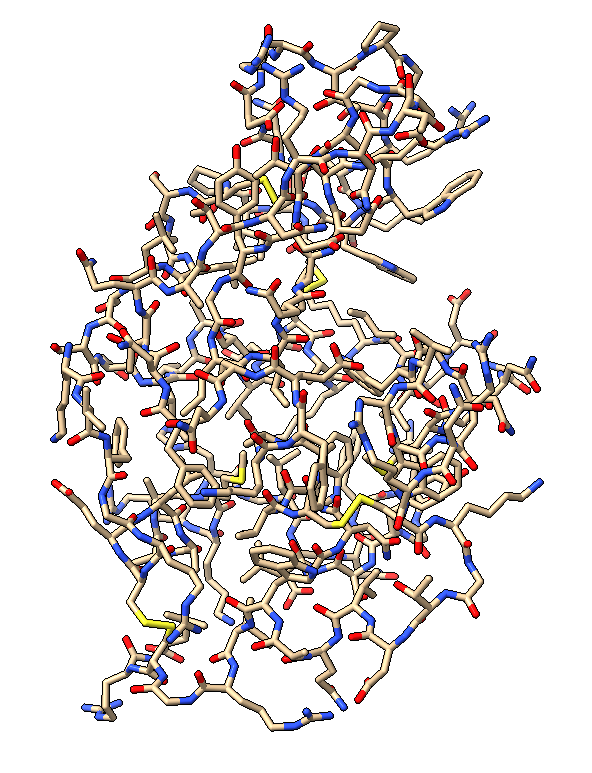
The first step in preparing a GROMACS simulation is to inspect and clean the starting structure. In this example, we begin with a lysozyme PDB file, which must be prepared in a GROMACS-compatible format before proceeding further. Classical lysozyme in water tutorials also start by downloading the appropriate PDB structure, visualizing it, and removing unnecessary elements, such as crystallographic water molecules.

The input file with the .pdb extension (1AKI.pdb) can be obtained from the PDB database (https://www.rcsb.org/) or downloaded directly into the desired directory:

wget https://files.rcsb.org/download/1AKI.pdb

When inspecting the initial PDB file, particular attention should be paid to the following points:

• whether the structure contains crystallographic water molecules (for example, HOH residues), which are typically removed in standard aqueous simulation workflows;

• whether the file contains ligands, cofactors, or other HETATM records that are not required for the present example;

• whether the PDB annotations indicate missing atoms or missing residues, as these may cause problems during the subsequent pdb2gmx step;

• whether the system contains only the macromolecule that is intended for simulation.

Visual inspection of the PDB file is recommended before starting any GROMACS operations. Any commonly used molecular visualization program can be used for this purpose. Lysozyme tutorials also recommend examining the structure first before proceeding to topology generation.

Crystallographic water molecules can most easily be removed with a text editor or from the command line. GROMACS tutorials typically assume that the input PDB contains only the protein atoms required for the simulation. Removing crystal waters is standard practice because the system will later be solvated again using a defined water model.

A typical command-line cleanup procedure is:

grep -v HOH 1AKI.pdb > 1AKI_clean.pdb

This command removes all lines containing the HOH identifier and creates a new cleaned PDB file (1AKI_clean.pdb). Other unwanted records can be filtered in a similar manner.

The purpose of preparing the input structure is therefore to ensure that, in the next step, pdb2gmx operates on a clean, consistent protein structure without missing or unnecessary components. This is a fundamental prerequisite for successful topology generation.

Topology Generation

Once the cleaned PDB file has been prepared, the next step is to generate the protein topology. In GROMACS, this is typically accomplished using the gmx pdb2gmx command, which generates a GROMACS-compatible coordinate file, a topology file, and, if required, position restraint files from the input protein structure.

In this example, the following command was used for topology generation:

gmx pdb2gmx -f 1AKI_clean.pdb -o 1AKI_processed.gro -water tip3p

In this command, the -f option specifies the input PDB file, -o specifies the output coordinate file in GROMACS format, and -water tip3p selects the water model. During the execution of pdb2gmx, the program asks which force field should be used; in this example, the CHARMM27 parameter set was selected.

According to the GROMACS documentation, CHARMM27 is an officially supported all-atom CHARMM force field available in GROMACS. The choice of force field determines the topology parameters, atom types, atomic charges, and bonded interactions. Consequently, it is important that all subsequent simulation settings remain consistent with this choice.

After running pdb2gmx, the following important files are typically generated:

• 1AKI_processed.gro → processed coordinate file in GROMACS format;

• topol.top → main topology file of the system;

• posre.itp → position restraint file for the protein, typically used during equilibration stages.

After topology generation, it is good practice to verify that the processed structure appears reasonable when visualized.

System Box Construction and Solvation

After generating the topology, the protein must be placed into a simulation box of appropriate size and the box must then be filled with solvent. In a typical GROMACS protein-in-water workflow, this is usually done using the gmx editconf and gmx solvate commands.

The goal of the box construction step is to ensure that there is sufficient distance between the protein and the box boundaries, thereby avoiding artificial interactions caused by periodic boundary conditions. For this reason, GROMACS tutorials typically define a minimum distance between the macromolecule and the box walls.

In this example, the following command was used to create the simulation box:

gmx editconf -f 1AKI_processed.gro -o 1AKI_newbox.gro -c -d 1.2 -bt cubic

In this command, -f specifies the input coordinate file, -o specifies the name of the output coordinate file, -c centers the protein in the box, and -d 1.2 requires a minimum distance of 1.2 nm between the protein and the box boundaries. The -bt cubic option sets the box shape to cubic.

After defining the box, the system must be filled with water molecules. In this example, the following command was used:

gmx solvate -cp 1AKI_newbox.gro -cs spc216.gro -o 1AKI_solv.gro -p topol.top

In this command, -cp specifies the coordinate file containing the boxed protein, -cs specifies the solvent configuration to be used, -o defines the coordinate file of the solvated system, and -p topol.top ensures that the topology file is automatically updated with the number of added solvent molecules.

After box construction and solvation, it is recommended to verify that:

• the 1AKI_newbox.gro file has been generated and contains the centered protein together with the box dimensions;

• the 1AKI_solv.gro file has been generated and contains the solvated system;

• the topol.top file has been updated with the number of solvent molecules;

• the distance between the protein and the box boundaries appears reasonable and the solvated system looks physically meaningful upon visual inspection.

Adding Ions

Once the solvated system has been generated, the next step is the addition of ions. The primary purpose of this step is to neutralize the net charge of the system and, if desired, to establish a specific salt concentration.

Before ions can be added, a .tpr run input file must be generated using gmx grompp. This is typically done using a simple energy-minimization-type ions.mdp file because the genion program requires a prepared system description.

A typical ions.mdp file is shown below:

; ions.mdp - used as input into grompp to generate ions.tpr
; Parameters describing what to do, when to stop and what to save
integrator  = steep         ; Algorithm (steep = steepest descent minimization)
emtol       = 1000.0        ; Stop minimization when the maximum force < 1000.0 kJ/mol/nm
emstep      = 0.01          ; Minimization step size
nsteps      = 50000         ; Maximum number of (minimization) steps to perform

; Parameters describing how to find the neighbors of each atom and how to calculate the interactions
nstlist         = 1         ; Frequency to update the neighbor list and long range forces
cutoff-scheme   = Verlet    ; Buffered neighbor searching
ns_type         = grid      ; Method to determine neighbor list (simple, grid)
coulombtype     = cutoff    ; Treatment of long range electrostatic interactions
rcoulomb        = 1.0       ; Short-range electrostatic cut-off
rvdw            = 1.0       ; Short-range Van der Waals cut-off
pbc             = xyz       ; Periodic Boundary Conditions in all 3 dimensions

A typical preparation command is:

gmx grompp -f ions.mdp -c 1AKI_solv.gro -p topol.top -o ions.tpr

In this command, -f specifies the ions.mdp parameter file, -c the solvated coordinate file, -p the topology file, and -o the binary run input file ions.tpr.

The ions can then be added using the gmx genion command. A simple example for charge neutralization is:

gmx genion -s ions.tpr -o 1AKI_solv_ions.gro -p topol.top -pname NA -nname CL -neutral

In this command, -s specifies the ions.tpr file generated by grompp, -o defines the output coordinate file, and -p topol.top ensures that the topology file is updated with the numbers of added ions. The -pname NA and -nname CL options define the names of the positive and negative ions, while -neutral instructs the program to neutralize the net charge of the system.

When the command is executed, the program asks which atom group should be partially replaced by ions. In this example, the SOL group with index 13 should be selected, meaning that water molecules are replaced by ions. This ensures that ions are inserted into the solvent rather than replacing protein atoms.

If the objective is not only to neutralize the system but also to reproduce a physiological salt concentration, the -conc option can be used. For example, -conc 0.150 requests an approximate salt concentration of 150 mM. When used together with -neutral, the system remains electrically neutral. This approach is commonly employed in protein-water simulation tutorials.

After ion addition, it is advisable to verify that the file 1AKI_solv_ions.gro has been generated and contains the newly added ions.

At this stage, the solvated and charge-neutralized system is ready for the energy minimization step.

Energy Minimization

The purpose of energy minimization is to remove unfavorable close contacts, steric clashes, and potentially poor local geometries from the system before starting the actual molecular dynamics simulations.

According to the GROMACS documentation, energy minimization can be performed using several algorithms, but for the preparation of biomolecular systems, the steepest descent method is one of the most common choices because it is robust and easy to apply. The algorithm runs until either a user-defined force threshold is reached or the maximum number of allowed steps is exhausted.

To perform energy minimization, a minim.mdp file is required. This file contains the minimization parameters, including the algorithm to be used (for example steep), the convergence criterion (emtol), the step size (emstep), and the maximum number of steps (nsteps). In other words, this file defines how GROMACS performs the energy minimization.

Example minim.mdp file:

; minim.mdp - used as input into grompp to generate em.tpr
; Parameters describing what to do, when to stop and what to save
integrator  = steep         ; Algorithm (steep = steepest descent minimization)
emtol       = 1000.0        ; Stop minimization when the maximum force < 1000.0 kJ/mol/nm
emstep      = 0.01          ; Minimization step size
nsteps      = 50000         ; Maximum number of (minimization) steps to perform

; Parameters describing how to find the neighbors of each atom and how to calculate the interactions
nstlist         = 1         ; Frequency to update the neighbor list and long range forces
cutoff-scheme   = Verlet    ; Buffered neighbor searching
ns_type         = grid      ; Method to determine neighbor list (simple, grid)
coulombtype     = PME       ; Treatment of long-range electrostatic interactions
rcoulomb        = 1.0       ; Short-range electrostatic cut-off
rvdw            = 1.0       ; Short-range Van der Waals cut-off
pbc             = xyz       ; Periodic Boundary Conditions in all 3 dimensions

In this example, integrator = steep selects the steepest descent algorithm, emtol = 1000.0 specifies the target maximum force threshold in kJ mol^-1nm^-1, emstep = 0.01 defines the maximum step size, and nsteps = 50000 sets the maximum number of allowed minimization steps. The settings for nonbonded interactions and periodic boundary conditions are also specified in this file.

To run the energy minimization, a .tpr input file must first be generated using the gmx grompp command.

gmx grompp -f minim.mdp -c 1AKI_solv_ions.gro -p topol.top -o em.tpr

In this command, -f specifies the energy minimization parameter file, -c specifies the initial coordinate file, -p specifies the topology file, and -o specifies the output binary run input file em.tpr. The purpose of grompp is to combine the coordinates, topology, and .mdp settings into a single simulation input file.

The minimization itself is then performed using the gmx mdrun command:

gmx mdrun -v -deffnm em

The -v option provides more detailed progress information on the screen, while -deffnm em specifies that all input and output files associated with the run will use em as the default filename prefix. According to the GROMACS documentation, mdrun can be used not only for molecular dynamics simulations but also for energy minimization if this is specified in the .tpr file.

The following files are typically generated during the run:

• em.tpr → binary run input file for the energy minimization;

• em.log → log file containing information about convergence and force values;

• em.edr → energy file from which energy components can later be extracted;

• em.gro → energy-minimized structure that will serve as the starting geometry for subsequent equilibration steps.

For a successful minimization, a message similar to the following should appear either in the terminal or near the end of the em.log file:

Steepest Descents converged to Fmax < 1000 in ... steps

This indicates that the steepest descent algorithm has reached the desired force threshold. The lysozyme tutorial considers this one of the most important signs of a successful energy minimization.

The following command can be used to extract the evolution of the potential energy into a potential.xvg file:

gmx energy -f em.edr -o potential.xvg

When running gmx energy, the values 11 0 should be entered at the prompt. Here, 11 selects the Potential energy term, while 0 ends the selection process.

The resulting data can be visualized using a short Python script (potential_plot.py).

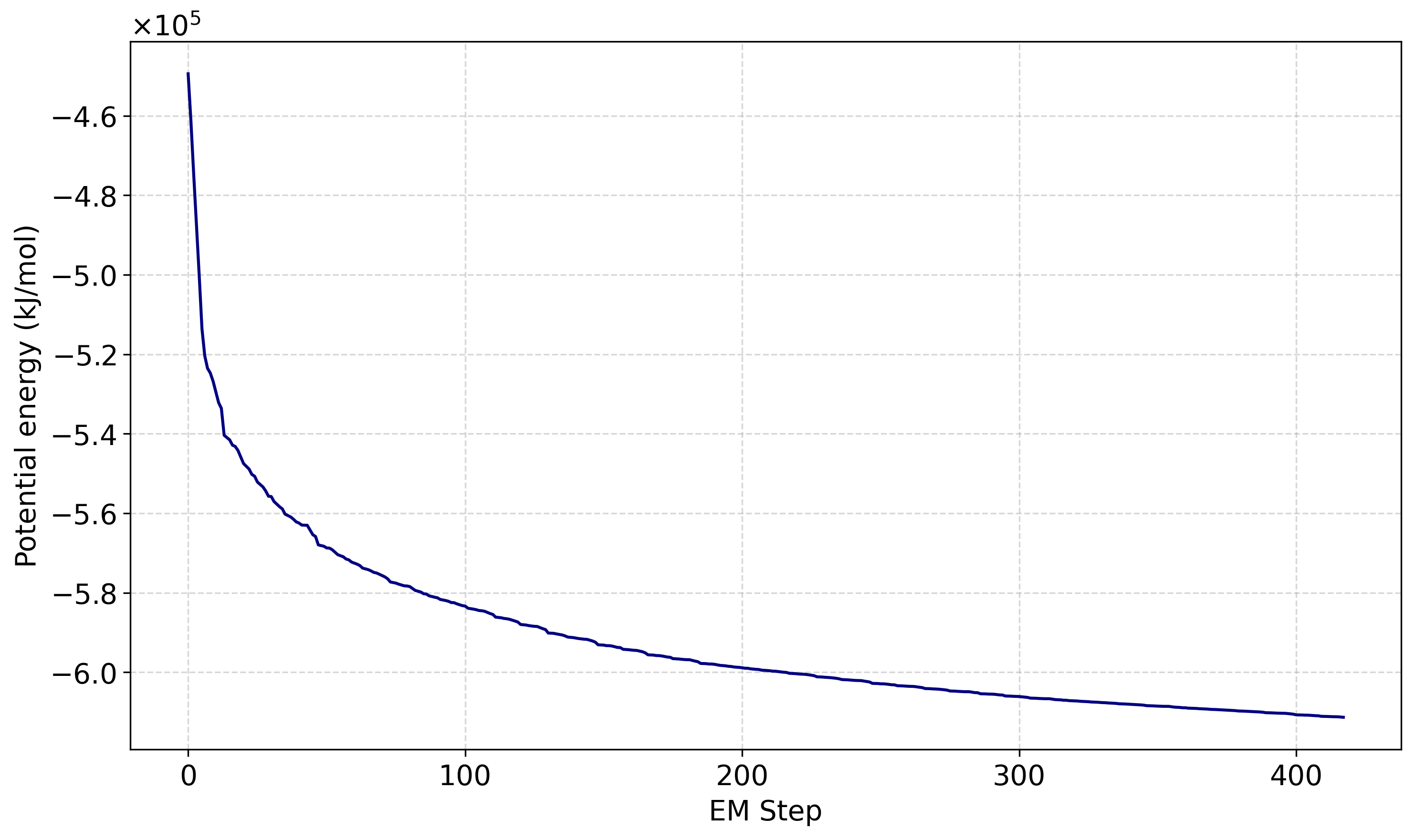
The energy-minimized structure stored in em.gro will serve as the starting geometry for the next step of the workflow, namely the NVT equilibration.

NVT Equilibration

After energy minimization, the system cannot yet be considered fully equilibrated. Although most geometric strain and steric clashes have already been removed, the water molecules and ions still need to adapt to the protein environment. During equilibration, we use the posre.itp file that was previously generated by pdb2gmx. According to the GROMACS documentation, the purpose of position restraints at this stage is to keep critical parts of the system, such as the protein heavy atoms, fixed in place while the solvent and ions reorganize around them.

The purpose of the NVT stage is to stabilize the temperature of the system at constant volume. According to the lysozyme tutorial, this phase is typically relatively short and is generally sufficient for the system to reach the target temperature. In this example, the NVT equilibration starts from the energy-minimized structure.

NVT equilibration requires an nvt.mdp file that contains the temperature equilibration parameters. The lysozyme tutorial specifically highlights several important settings used at this stage, including gen_vel = yes, which generates initial velocities, tcoupl = V-rescale, which controls the temperature, and pcoupl = no, because pressure coupling is not yet applied during this stage.

Example nvt.mdp file:

title                   = OPLS Lysozyme NVT equilibration
define                  = -DPOSRES  ; position restrain the protein
; Run parameters
integrator              = md        ; leap-frog integrator
nsteps                  = 50000     ; 2 * 50000 = 100 ps
dt                      = 0.002     ; 2 fs
; Output control
nstxout                 = 2500      ; save coordinates every 5.0 ps
nstvout                 = 2500      ; save velocities every 5.0 ps
nstenergy               = 2500      ; save energies every 5.0 ps
nstlog                  = 2500      ; update log file every 5.0 ps
; Bond parameters
continuation            = no        ; first dynamics run
constraint_algorithm    = lincs     ; holonomic constraints
constraints             = h-bonds   ; bonds involving H are constrained
lincs_iter              = 1         ; accuracy of LINCS
lincs_order             = 4         ; also related to accuracy
; Nonbonded settings
cutoff-scheme           = Verlet    ; Buffered neighbor searching
ns_type                 = grid      ; search neighboring grid cells
nstlist                 = 10        ; 20 fs, largely irrelevant with Verlet
; vdW
rvdw                    = 1.2       ; short-range van der Waals cutoff (in nm)
rvdw-switch             = 1.0
vdw-modifier            = force-switch
DispCorr                = No        ; per CHARMM FF convention
; Electrostatics
rcoulomb                = 1.2       ; short-range electrostatic cutoff (in nm)
coulombtype             = PME       ; Particle Mesh Ewald for long-range electrostatics
pme_order               = 4         ; cubic interpolation
fourierspacing          = 0.16      ; grid spacing for FFT
; Temperature coupling is on
tcoupl                  = V-rescale ; stochastic Bussi thermostat
tc-grps                 = System
tau_t                   = 1.0       ; value of tau (ps)
ref_t                   = 298       ; temperature (K)
; Pressure coupling is off
pcoupl                  = no        ; no pressure coupling in NVT
; Periodic boundary conditions
pbc                     = xyz       ; 3-D PBC
; Velocity generation
gen_vel                 = yes       ; assign velocities from Maxwell distribution
gen_temp                = 298       ; temperature for Maxwell distribution
gen_seed                = -1        ; generate a random seed

Before running the NVT equilibration, a run input file nvt.tpr must be generated:

gmx grompp -f nvt.mdp -c em.gro -r em.gro -p topol.top -o nvt.tpr

In this command, the -f option specifies the NVT parameter file, -c em.gro specifies the energy-minimized structure, and -r em.gro provides the reference coordinates for the position restraints. The lysozyme tutorial explicitly emphasizes that restrained equilibration requires the use of the -r option to define the coordinate file relative to which the restraints are applied.

The NVT simulation can then be started using the following command:

gmx mdrun -deffnm nvt

The -deffnm nvt option instructs GROMACS to create all input and output files using the prefix nvt, such as nvt.log, nvt.edr, nvt.cpt, and nvt.gro. The mdrun program is the general execution engine of GROMACS, which performs the simulation according to the instructions contained in the .tpr file. After the NVT run, it is important to verify that the system temperature has stabilized properly.

The evolution of the temperature can be extracted to a temperature.xvg file using the following command:

gmx energy -f nvt.edr -o temperature.xvg

When running gmx energy, the values 16 0 should be entered at the prompt. Here, 16 selects the system Temperature term, while 0 finalizes the selection.

The resulting data can then be visualized using a short Python script (temperature_plot.py).

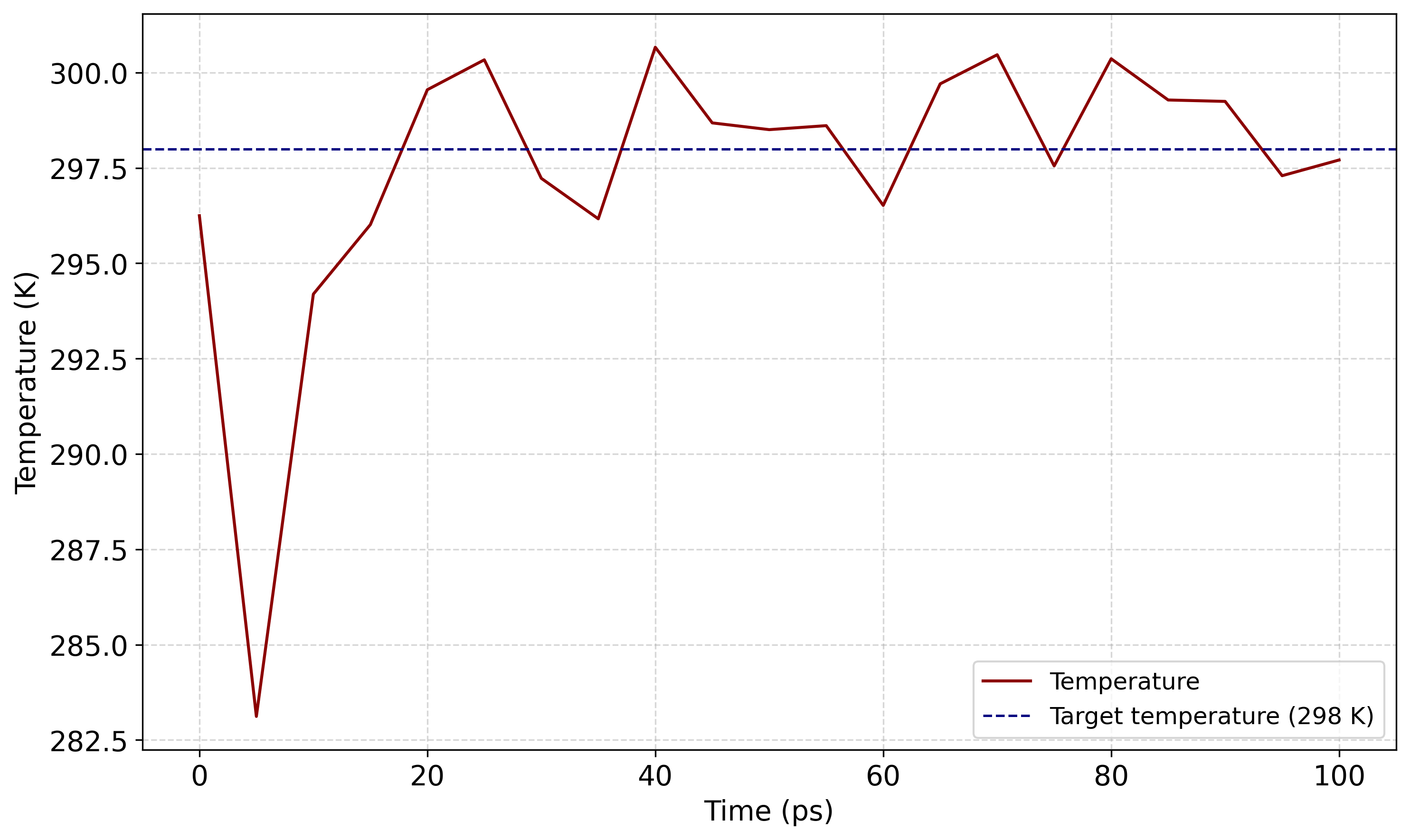
A successful NVT equilibration is indicated by the temperature fluctuating around the target value (298 K in this example) without exhibiting systematic drift. The structure stored in nvt.gro together with the checkpoint file nvt.cpt will serve as the starting point for the subsequent NPT equilibration stage.

NPT Equilibration

The next step is NPT equilibration, whose purpose is to stabilize the pressure and, consequently, the density of the system.

Running the NPT stage requires an npt.mdp file, which, in addition to the parameters used during NVT equilibration, also contains settings for pressure coupling. At this stage, it is important to continue the simulation from the NVT run; therefore, the typical settings include continuation = yes and gen_vel = no. In this phase, new velocities are not generated. Instead, the velocities obtained in the previous stage are used.

Example npt.mdp file:

title                   = OPLS Lysozyme NPT equilibration
define                  = -DPOSRES  ; position restrain the protein
; Run parameters
integrator              = md        ; leap-frog integrator
nsteps                  = 250000    ; 2 * 250000 = 500 ps
dt                      = 0.002     ; 2 fs
; Output control
nstxout                 = 500       ; save coordinates every 1.0 ps
nstvout                 = 500       ; save velocities every 1.0 ps
nstenergy               = 500       ; save energies every 1.0 ps
nstlog                  = 500       ; update log file every 1.0 ps
; Bond parameters
continuation            = yes       ; Restarting after NVT
constraint_algorithm    = lincs     ; holonomic constraints
constraints             = h-bonds   ; bonds involving H are constrained
lincs_iter              = 1         ; accuracy of LINCS
lincs_order             = 4         ; also related to accuracy
; Nonbonded settings
cutoff-scheme           = Verlet    ; Buffered neighbor searching
ns_type                 = grid      ; search neighboring grid cells
nstlist                 = 10        ; 20 fs, largely irrelevant with Verlet scheme
; vdW
rvdw                    = 1.2       ; short-range van der Waals cutoff (in nm)
rvdw-switch             = 1.0
vdw-modifier            = force-switch
DispCorr                = No
; Electrostatics
rcoulomb                = 1.2       ; short-range electrostatic cutoff (in nm)
coulombtype             = PME       ; Particle Mesh Ewald for long-range electrostatics
pme_order               = 4         ; cubic interpolation
fourierspacing          = 0.16      ; grid spacing for FFT
; Temperature coupling is on
tcoupl                  = V-rescale ; stochastic Bussi thermostat
tc-grps                 = System
tau_t                   = 1.0
ref_t                   = 298
; Pressure coupling is on
pcoupl                  = C-rescale
pcoupltype              = isotropic             ; uniform scaling of box vectors
tau_p                   = 5.0                   ; time constant, in ps
ref_p                   = 1.0                   ; reference pressure, in bar
compressibility         = 4.5e-5                ; isothermal compressibility of water, bar^-1
refcoord_scaling        = com
; Periodic boundary conditions
pbc                     = xyz       ; 3-D PBC
; Velocity generation
gen_vel                 = no        ; Velocity generation is off

The NPT run input file (npt.tpr) can be generated using the following command:

gmx grompp -f npt.mdp -c nvt.gro -r nvt.gro -t nvt.cpt -p topol.top -o npt.tpr

In this command, -c nvt.gro specifies the final coordinates obtained from the NVT equilibration, -r nvt.gro still provides the reference structure for the position restraints, while -t nvt.cpt ensures that the system state continues seamlessly from the NVT stage.

The NPT simulation is started with:

gmx mdrun -deffnm npt

The run typically generates the files npt.gro, npt.edr, npt.log, and npt.cpt.

Among these, npt.gro will serve as the starting structure for the production simulation, while npt.cpt contains the simulation state required to restart or continue the run later. After NPT equilibration, it is advisable to verify that the system density and pressure have stabilized to reasonable values.

The pressure profile can be extracted into a pressure.xvg file using the following command:

gmx energy -f npt.edr -o pressure.xvg

When running gmx energy, enter the values 17 0 at the prompt. Here, 17 selects the system Pressure term, while 0 finalizes the selection.

The resulting data can then be plotted using a short Python script (pressure_plot.py).

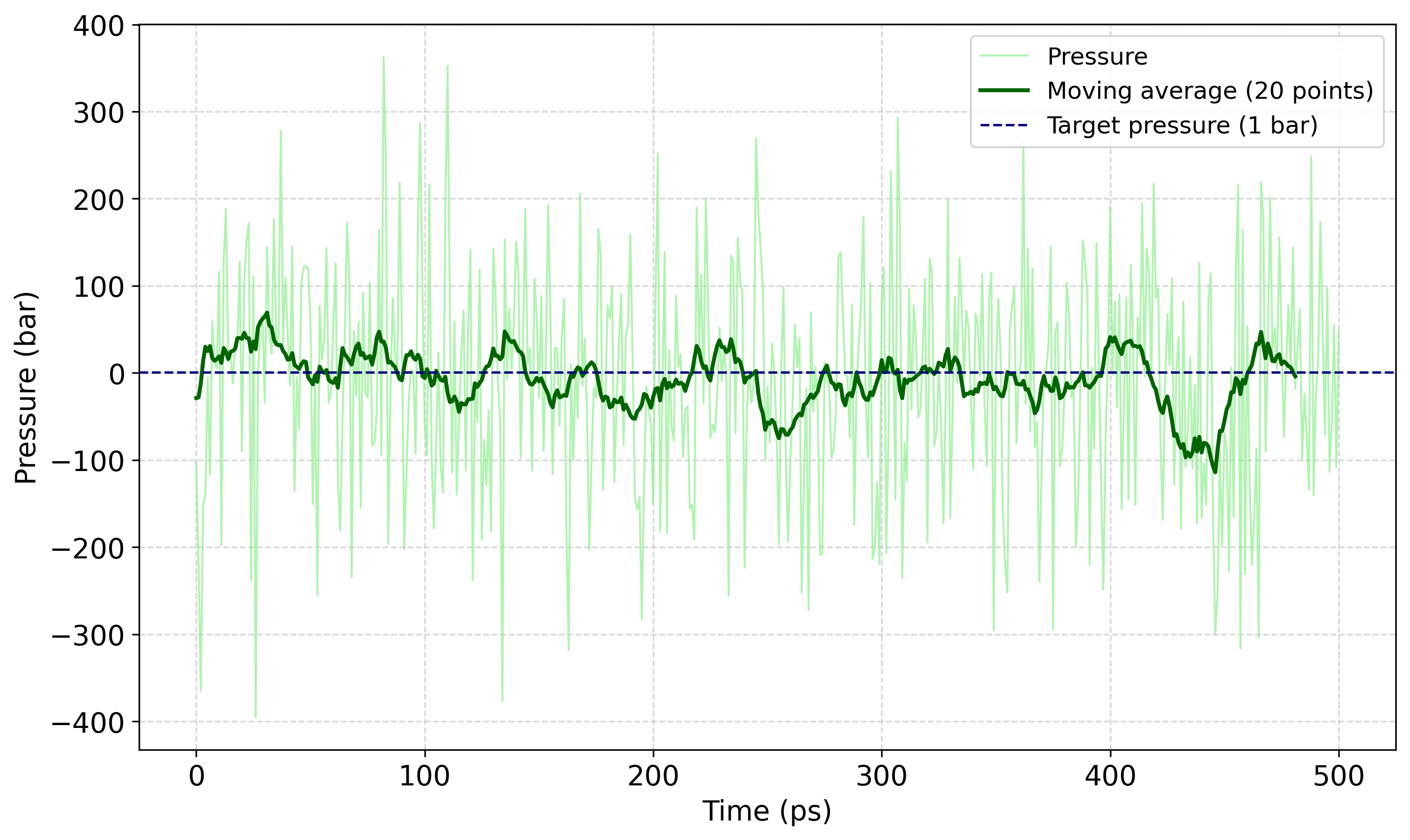
Unlike the temperature, the instantaneous pressure typically exhibits large fluctuations during molecular dynamics simulations. Therefore, the average pressure and its long-term behavior are generally more informative than the instantaneous values themselves. If the average pressure remains close to the target value and the density has converged to a stable value, the NPT equilibration can be considered successful.

The equilibrated structure stored in npt.gro is then ready to be used as the starting point for the production molecular dynamics simulation.

Production Run

After the two equilibration stages, the system is properly stabilized at the desired temperature and pressure. Therefore, the position restraints can be removed and the production molecular dynamics simulation can begin. Running the production stage requires an md.mdp file that contains the parameters for a longer, unrestrained molecular dynamics simulation.

Example md.mdp file:

title                   = OPLS Lysozyme MD run
; Run parameters
integrator              = md        ; leap-frog integrator
nsteps                  = 5000000   ; 2 * 2500000 = 10000 ps (10 ns)
dt                      = 0.002     ; 2 fs
; Output control
nstxout                 = 0         ; suppress bulky .trr file by specifying
nstvout                 = 0         ; 0 for output frequency of nstxout,
nstfout                 = 0         ; nstvout, and nstfout
nstenergy               = 5000      ; save energies every 10.0 ps
nstlog                  = 5000      ; update log file every 10.0 ps
nstxout-compressed      = 5000      ; save compressed coordinates every 10.0 ps
compressed-x-grps       = System    ; save the whole system
; Bond parameters
continuation            = yes       ; Restarting after NPT
constraint_algorithm    = lincs     ; holonomic constraints
constraints             = h-bonds   ; bonds involving H are constrained
lincs_iter              = 1         ; accuracy of LINCS
lincs_order             = 4         ; also related to accuracy
; Nonbonded settings
cutoff-scheme           = Verlet    ; Buffered neighbor searching
ns_type                 = grid      ; search neighboring grid cells
nstlist                 = 10        ; 20 fs, largely irrelevant with Verlet scheme
; vdW
rvdw                    = 1.2       ; short-range van der Waals cutoff (in nm)
rvdw-switch             = 1.0
vdw-modifier            = force-switch
DispCorr                = No
; Electrostatics
rcoulomb                = 1.2       ; short-range electrostatic cutoff (in nm)
coulombtype             = PME       ; Particle Mesh Ewald for long-range electrostatics
pme_order               = 4         ; cubic interpolation
fourierspacing          = 0.16      ; grid spacing for FFT
; Temperature coupling is on
tcoupl                  = V-rescale             ; modified Berendsen thermostat
tc-grps                 = System
tau_t                   = 1.0
ref_t                   = 298
; Pressure coupling is on
pcoupl                  = C-rescale
pcoupltype              = isotropic             ; uniform scaling of box vectors
tau_p                   = 5.0                   ; time constant, in ps
ref_p                   = 1.0                   ; reference pressure, in bar
compressibility         = 4.5e-5                ; isothermal compressibility of water, bar^-1
; Periodic boundary conditions
pbc                     = xyz       ; 3-D PBC
; Velocity generation
gen_vel                 = no        ; Velocity generation is off

Preparation of the run input file (md.tpr):

gmx grompp -f inputs/md.mdp -c npt.gro -t npt.cpt -p topol.top -o md.tpr

In this command, -c npt.gro specifies the final structure obtained from the NPT equilibration, while -t npt.cpt provides the checkpoint file required for a continuous continuation of the simulation.

Starting the production simulation:

gmx mdrun -deffnm md

During the simulation, GROMACS generates the standard output files associated with a production molecular dynamics run, including the log file, energy file, final coordinate file, and checkpoint file. Since the default filename prefix is md, these files are created with the corresponding prefix.

According to the GROMACS documentation, mdrun executes the task defined in the .tpr input file and generates the associated output files, including md.log, md.edr, md.gro, and md.cpt.

The trajectory itself is stored in md.xtc.

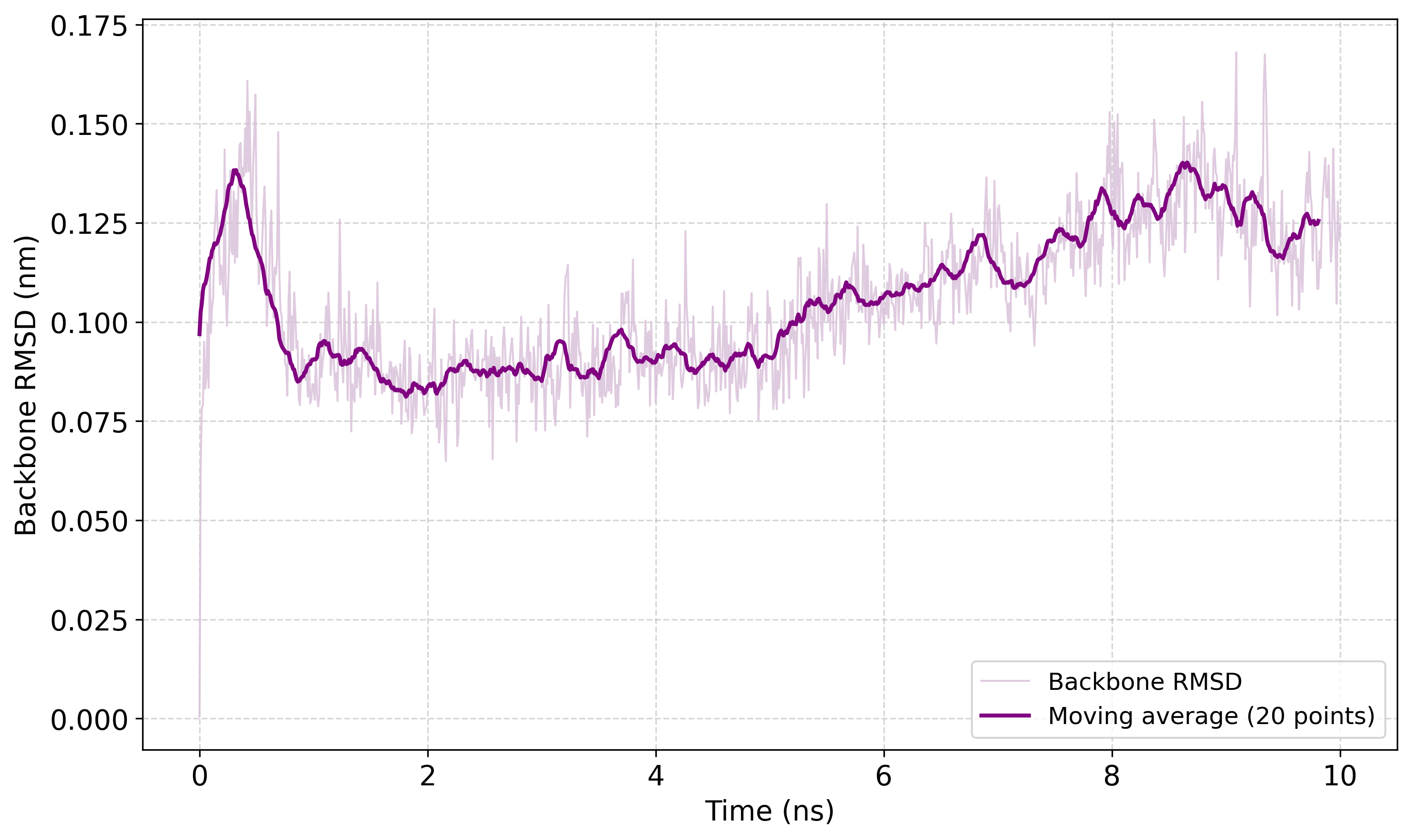
Analysis: Backbone RMSD Calculation

After the production simulation, one of the simplest and most commonly used structural analyses is the calculation of the backbone RMSD. Before performing the RMSD calculation, it is recommended to preprocess the trajectory so that periodic boundary conditions do not distort the results. This is necessary because the protein may diffuse within the simulation box during the run, causing the trajectory to appear fragmented or artificially displaced.

Periodic boundary effects can be corrected using the gmx trjconv command:

gmx trjconv -s md.tpr -f md.xtc -o md_PBC.xtc -pbc mol -center

According to the tutorial, when running this command, the Protein group (index 1) should first be selected for centering, followed by the System group (index 0) for outputting the complete system. The resulting trajectory md_PBC.xtc is free from the most prominent visual and geometric artifacts caused by periodicity, making it more suitable for further analysis.

The backbone RMSD can then be calculated using the gmx rms command:

gmx rms -s md_0_10.tpr -f md_0_10_noPBC.xtc -o rmsd.xvg -tu ns

According to the tutorial, the Backbone group (index 4) should be selected both for the least-squares fitting step and for the RMSD calculation itself. The -tu ns option specifies that the time axis should be displayed in nanoseconds, which is generally more convenient than picoseconds when working with longer trajectories.

The resulting rmsd.xvg file contains the backbone RMSD values as a function of simulation time. According to the lysozyme tutorial, this curve provides information about how much the protein backbone deviates from the reference structure during the simulation. In this example, the reference structure corresponds to the minimized and equilibrated system represented by md_0_10.tpr.

The rmsd.xvg data can later be visualized using a short Python script (rmsd_plot.py).