AMBER

Obtaining and Preparing the PDB File

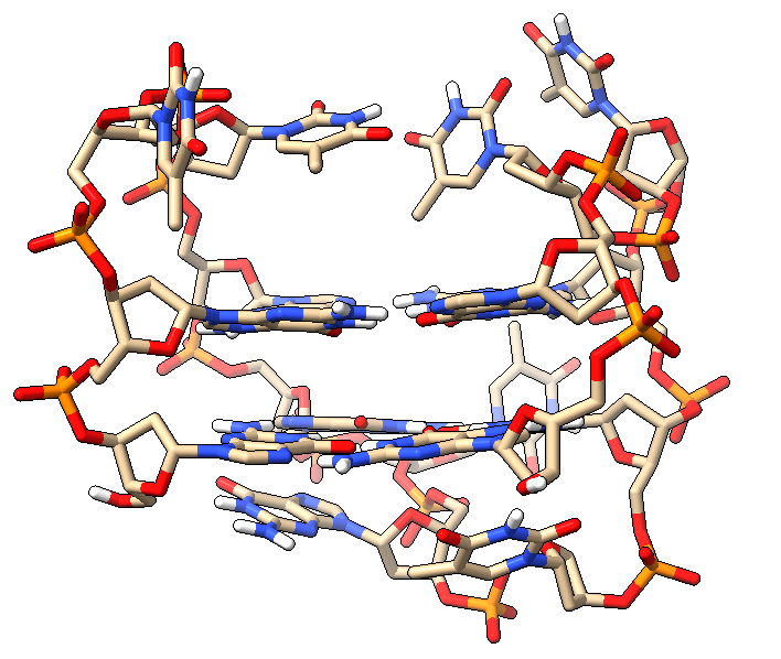
For this AMBER example, we use a thrombin-binding DNA aptamer, a single-stranded 15-nucleotide DNA aptamer whose structure was determined by solution NMR. The PDB identifier of the structure is 1RDE. According to the PDB entry, the structure is provided as an NMR ensemble consisting of 11 conformers. In the following examples, only the first model will be used.

The input file with the .pdb extension can be obtained from the PDB database (https://www.rcsb.org/) or downloaded directly into the desired directory as follows:

wget https://files.rcsb.org/download/1RDE.pdb

This PDB file contains NMR ensemble information and may also include records or formatting elements that are not ideal for further processing with LEaP/AMBER. A properly formatted PDB file suitable for subsequent calculations can be generated using the pdb4amber program:

pdb4amber -i 1RDE.pdb -o 1RDE_clean.pdb

Files: 1RDE.pdb, 1RDE_clean.pdb

Generating Topology and Coordinate Files with LEaP

The AMBER program LEaP can be used to generate topology and coordinate files. During system setup, an appropriate force field and solvent model must also be selected. The force fields recommended for a given AMBER version and the available solvent models are described in the AMBER manual (https://ambermd.org/Manuals.php).

In this example, we use the OL21 force field recommended for nucleic acids and the OPC water model. Since the phosphate backbone of the structure carries a negative charge, positively charged counterions must be added to neutralize the system. The addition of counterions ensures that the total charge of the system is neutral.

Example tleap script (tleap_1RDE.in):

source leaprc.DNA.OL21
source leaprc.water.opc

mol = loadpdb 1RDE_clean.pdb
check mol
charge mol

addions mol Na+ 14
solvatebox mol OPCBOX 10.0

saveamberparm mol 1RDE.prmtop 1RDE.rst7
quit

In the first two lines, we load the selected force field and solvent model. Next, we load the .pdb file and refer to the resulting system as mol. The check command performs a basic structural validation, while charge prints the total charge of the system.

The addions command adds the number of sodium ions required to neutralize the net charge of the system. The solvatebox command places the structure in an explicit solvent box such that the walls of the box are at least 10 Å away from the outermost atoms of the system.

Finally, the saveamberparm command saves the topology (.prmtop) and coordinate (.rst7) files required for subsequent calculations.

The tleap script can be executed as follows:

tleap -f tleap_1RDE.in

Any issues encountered during the execution of tleap, as well as a detailed record of the performed steps, can be found in the leap.log file.

If tleap completes successfully and the 1RDE.prmtop and 1RDE.rst7 files have been generated, we can proceed with the molecular dynamics calculations.

Energy Minimization

The initial structure generated by LEaP does not necessarily correspond exactly to a local energy minimum of the selected force field. In addition, after solvation and the addition of ions, the system may contain unfavorable contacts, overlapping atoms, short interatomic distances, or locally strained regions. Therefore, an energy minimization step is performed before starting the molecular dynamics simulation.

The purpose of energy minimization is to allow the system to relax toward the nearest local minimum and eliminate unfavorable interactions that might lead to instabilities during the subsequent heating or production simulation. This step is not intended to locate the global energy minimum, but rather to ensure that the starting structure is physically reasonable.

For solvated systems, it is generally recommended to perform minimization in two stages. In the first stage, positional restraints are applied to the biomolecule, allowing primarily the water molecules and ions to relax around the structure. In the second stage, the restraints are reduced or removed entirely, enabling the whole system to relax further.

In an AMBER minimization input file, imin=1 activates energy minimization. The maxcyc parameter specifies the maximum number of minimization cycles, while ntmin=1 applies the steepest descent algorithm during the first ncyc steps and the conjugate gradient algorithm during the remaining steps. The ntr=1 option enables positional restraints, restraint_wt defines their strength, and restraintmask specifies which atoms or residues are affected.

The restrained minimization input file (1_Min_rest.in):

Initial minimization with restraints
&cntrl
imin=1,
ntmin=1,
maxcyc=5000,
ncyc=2500,
ntb=1,
cut=10.0,
ntr=1,
restraint_wt=5.0,
restraintmask=':1-15',
/

This calculation can be run with either sander or pmemd as follows:

sander -O -i 1_Min_rest.in -o 1_Min_rest.out -p 1RDE.prmtop -c 1RDE.rst7 -r 1_Min_rest.rst7 -ref 1RDE.rst7

The -O option allows existing output files to be overwritten. The -i option specifies the input file, while -o defines the name of the text output file generated during the run. The -p option specifies the topology (parameter) file, and -c identifies the file containing the initial coordinates. The -r option defines the restart file that will contain the minimized coordinates at the end of the calculation.

Because positional restraints are applied during this step, the -ref option must also be provided to specify the reference coordinate file relative to which the restraints are interpreted.

Output files: 1_Min_rest.out, 1_Min_rest.rst7

This is followed by an unrestrained minimization (1_Min.in).

Unrestrained minimization
&cntrl
imin=1,
ntmin=1,
maxcyc=5000,
ncyc=2500,
ntb=1,
cut=10.0,
ntr=0,
/

The calculation is run using the same command as described previously, with the appropriate file names:

sander -O -i 1_Min.in -o 1_Min.out -p 1RDE.prmtop -c 1_Min_rest.rst7 -r 1_Min.rst7

After successful completion of the minimization step, the 1_Min.out file can be used to monitor the progress of the run and the evolution of the system energy, while the 1_Min.rst7 file contains the minimized coordinates.

The minimization can be considered successful if the calculation completes without errors, the system energy shows a decreasing trend, and no abnormal values appear in the output, such as NaN, ********, or extremely large nonbonded interaction energies. Such issues usually indicate bad contacts or an incorrect starting geometry.

Once the 1_Min.out file and the resulting structure have been inspected and the minimization has been judged successful, the next phase of the workflow, system heating, can begin.

System Heating

Following energy minimization, the system is gradually heated to the target temperature. The purpose of the heating stage is to bring the system to the desired simulation temperature without introducing sudden, high-energy motions into the structure. Excessively rapid heating may lead to instabilities; therefore, the temperature is increased gradually.

Heating is typically performed under constant-volume (NVT) conditions. During this stage, it is advisable to maintain weak positional restraints on the biomolecule so that the solvent molecules and ions can relax around the structure.

The following input file (2_Heat.in) can be used for heating:

Heating the system from 0 K to 300 K
&cntrl
imin=0,
irest=0,
ntx=1,
nstlim=25000,
dt=0.002,
ntc=2,
ntf=2,
tempi=0.0,
temp0=300.0,
ntpr=500,
ntwx=500,
ntwr=5000,
ntb=1,
ntp=0,
cut=10.0,
ntt=3,
gamma_ln=1.0,
ig=-1,
ntr=1,
restraint_wt=2.0,
restraintmask=':1-15',
nmropt=1,
/
&wt
type='TEMP0', istep1=0, istep2=20000, value1=0.0, value2=300.0,
/
&wt
type='TEMP0', istep1=20001, istep2=25000, value1=300.0, value2=300.0,
/
&wt type='END' /

The above example follows the typical structure of AMBER heating inputs:

imin=0 → molecular dynamics run rather than minimization
irest=0, ntx=1 → start a new simulation from coordinates without velocities
nstlim=25000, dt=0.002 → 50 ps simulation time
ntb=1, ntp=0 → constant volume (NVT), without pressure coupling
ntpr=500, ntwx=500, ntwr=5000 → energy and run information are written to the output file every 500 steps; coordinates are saved to the trajectory every 500 steps; the restart file is updated every 5000 steps
ntt=3, gamma_ln=1.0 → Langevin thermostat
nmropt=1 + &wt blocks → gradual temperature ramp from 0 K to 300 K

Command used to run the simulation:

sander -O -i 2_Heat.in -o 2_Heat.out -p 1RDE.prmtop -c 1_Min.rst7 -r 2_Heat.rst7 -x 2_Heat.nc -ref 1_Min.rst7

The success of the heating stage can be verified from the 2_Heat.out file. Heating can be considered successful if the system temperature approaches the target value gradually, the run completes without errors, and no abnormal values such as NaN or ******** appear in the output. It is also advisable to inspect the resulting trajectory (2_Heat.nc) visually to ensure that the nucleic acid structure does not undergo unrealistic distortions and that the solvent box behaves properly. The resulting 2_Heat.rst7 file may then be used as input for the subsequent equilibration stage.

Equilibration

After heating, the system is equilibrated under constant-pressure conditions. The purpose of this stage is to allow the size and density of the solvent box, as well as the arrangement of solvent molecules and ions, to adapt to the nucleic acid structure.

In explicit-solvent AMBER simulations, equilibration is typically started from the coordinates and velocities obtained at the end of the heating stage and is therefore performed as a restart run. During this phase, the system remains at the target temperature while pressure regulation allows the simulation box to adjust to the appropriate density.

The following input file (3_Equil.in) can be used for equilibration:

Equilibration at 300 K and 1 atm without restraints
&cntrl
imin=0,
irest=1,
ntx=5,
nstlim=50000,
dt=0.002,
ntc=2,
ntf=2,
temp0=300.0,
ntpr=500,
ntwx=500,
ntwr=5000,
ntb=2,
ntp=1,
taup=2.0,
cut=10.0,
ntt=3,
gamma_ln=1.0,
ig=-1,
ntr=0,
/

This equilibration run uses typical AMBER parameters:

imin=0 → molecular dynamics run, not energy minimization
irest=1, ntx=5 → restart simulation using the coordinates and velocities obtained after heating
nstlim=50000, dt=0.002 → 100 ps simulation time
ntb=2, ntp=1 → constant-pressure (NPT) simulation allowing box-size fluctuations
taup=2.0 → pressure relaxation time
temp0=300.0 → target temperature of 300 K
ntt=3, gamma_ln=1.0 → Langevin thermostat for temperature regulation
ntc=2, ntf=2 → constraints on bonds involving hydrogen atoms, allowing a 2 fs time step
ntr=0 → positional restraints are no longer applied during this stage
ntpr=500, ntwx=500, ntwr=5000 → energy and run information are written every 500 steps, coordinates are saved every 500 steps, and the restart file is updated every 5000 steps

Command used to run the equilibration:

sander -O -i 3_Equil.in -o 3_Equil.out -p 1RDE.prmtop -c 2_Heat.rst7 -r 3_Equil.rst7 -x 3_Equil.nc

Output files: 3_Equil.out, 3_Equil.nc, 3_Equil.rst7

At the end of the equilibration stage, it should be verified that the simulation completed successfully and that all expected output files were generated. The behavior of the density, temperature, and box dimensions can be used to assess whether the system is approaching equilibrium. Since the OPC water model is used in this example, and this model was specifically developed to accurately reproduce the bulk properties of liquid water, including its density, the equilibrated density of a solvated biomolecular system should also be close to that of liquid water, approximately 1.0 g/cm^3. Small deviations are expected due to the presence of the biomolecule and ions.

It is also important to verify that no NaN or ******** values appear in the output and that the trajectory exhibits physically reasonable structural behavior. If these conditions are satisfied, the system is ready for the production simulation stage.

Production Stage

After successful completion of the equilibration stage, the next step is to start the production run. During this phase, the system evolves at the desired temperature and pressure without positional restraints, making the resulting trajectory suitable for the analysis of structural and dynamic properties. The production run starts from the coordinates and velocities obtained at the end of equilibration and is therefore performed as a restart simulation.

An example 4_MD.in file for a 25 ns simulation is shown below:

Production MD at 300 K and 1 atm
&cntrl
imin=0,
irest=1,
ntx=5,
nstlim=12500000,
dt=0.002,
ntc=2,
ntf=2,
temp0=300.0,
ntpr=10000,
ntwx=10000,
ntwr=500000,
ioutfm=1,
ntb=2,
pres0=1.0,
ntp=1,
taup=2.0,
cut=10.0,
ntt=3,
gamma_ln=1.0,
ig=-1,
ntr=0,
/

The above production run uses typical AMBER settings:

imin=0 → molecular dynamics simulation, not energy minimization
irest=1, ntx=5 → restart simulation using previously generated coordinates and velocities
nstlim=12500000, dt=0.002 → 25 ns simulation time
ntb=2, ntp=1 → constant-pressure (NPT) simulation
temp0=300.0 → target temperature of 300 K
ntt=3, gamma_ln=1.0 → Langevin thermostat
ntr=0 → no positional restraints
ioutfm=1 → NetCDF trajectory format

Command required to run 4_MD.in:

pmemd -O -i 4_MD.in -o 4_MD.out -p 1RDE.prmtop -c 3_Equil.rst7 -r 4_MD.rst7 -x 4_MD.nc -inf 4_MD.mdinfo

Note

The simulation engine should be selected according to the available hardware. For general CPU-based simulations, either sander or the performance-optimized pmemd can be used. On GPU-equipped systems, pmemd.cuda is recommended, as it is AMBER’s GPU-optimized molecular dynamics engine. Parallel execution on multiple CPU cores in an MPI environment is typically performed using pmemd.MPI or sander.MPI.

Several important output files are generated during the simulation:

4_MD.out → detailed text log of the simulation
4_MD.rst7 → restart file generated at the end of the run
4_MD.nc → trajectory file
mdinfo → concise summary of the current simulation status during execution

Analysis: Trajectory RMSD and Hydrogen Bond Count Using cpptraj

As a first analysis, the RMSD of the trajectory can be calculated using the cpptraj program. Before performing the calculation, it is advisable to re-image the trajectory using the autoimage command so that systems that appear fragmented due to periodic boundary conditions are reconstructed into a physically meaningful representation. The RMSD can then be calculated relative to the first frame or to a separate reference structure. The trajout command can also be used to save a new, visually cleaner trajectory.

The following example calculates the RMSD of only the non-hydrogen atoms of the nucleic acid (cpptraj_rmsd.in):

parm 1RDE.prmtop
trajin 4_MD.nc

autoimage

rms first :1-15&!@H= out rmsd_1RDE.dat

trajout 4_MD_autoimaged.nc netcdf

run
quit

The RMSD can then be visualized using the following Python script (rmsd_plot.py):

import matplotlib.pyplot as plt

frames = []
rmsd = []

with open("rmsd_1RDE.dat") as f:
    for line in f:
        if line.strip() and not line.startswith("#"):
            parts = line.split()
            frames.append(int(parts[0]))
            rmsd.append(float(parts[1]))

# Create plot
plt.figure(figsize=(8,5))
plt.plot(frames, rmsd, color='blue', linewidth=2)
plt.xlabel("Frame")
plt.ylabel("RMSD [Å]")
plt.title("TBA tetrad RMSD during MD simulation")
plt.grid(True)
plt.tight_layout()
plt.savefig("rmsd_tetrad_plot.png", dpi=300)
plt.show()

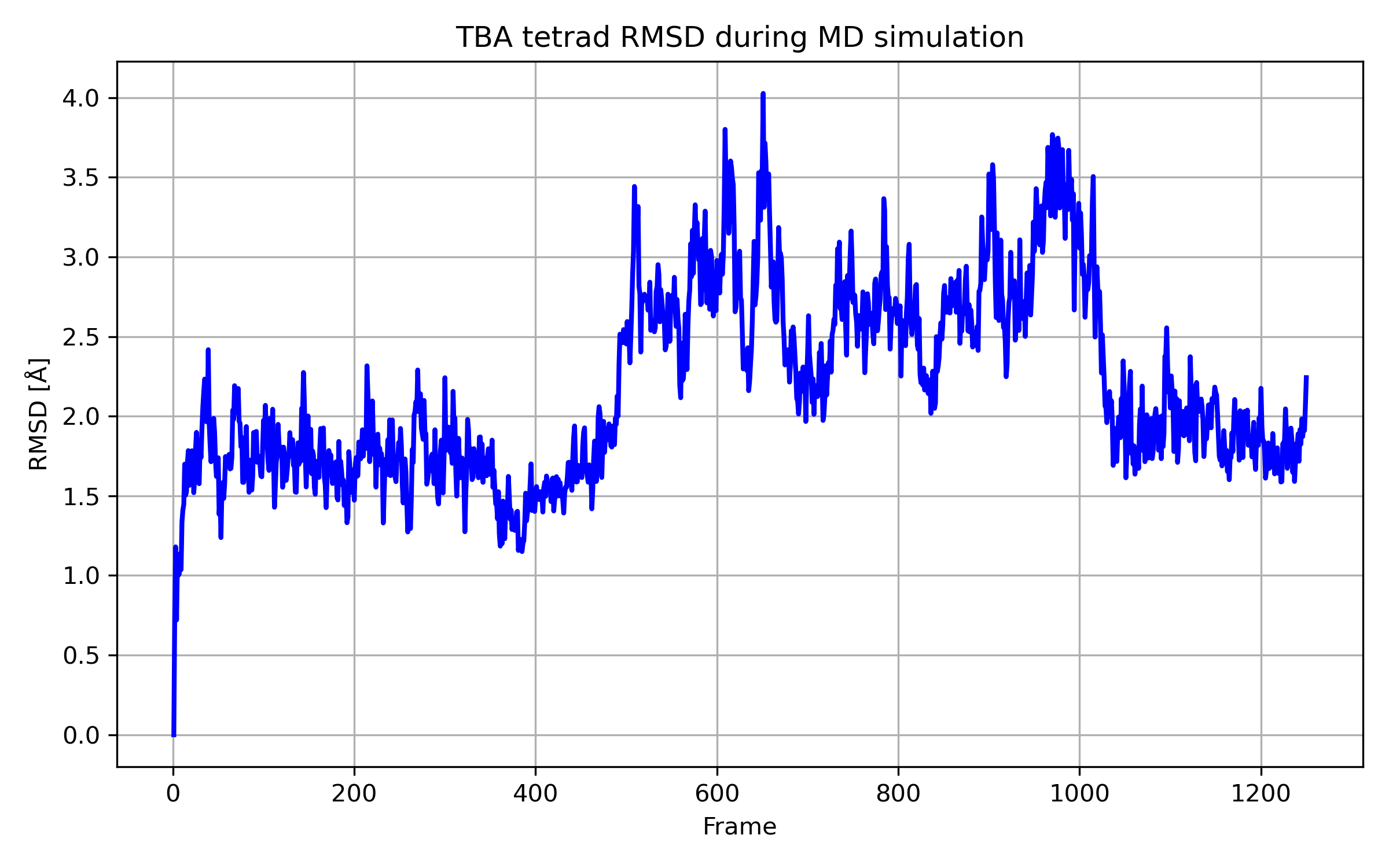
After visualizing the trajectory, the resulting RMSD profile provides a reasonable picture of the system’s behavior. During the simulation, the structure begins to partially unfold, and during the final 5 ns it returns to a geometry similar to the initial structure, where the tetrads are stabilized by secondary hydrogen-bond interactions.

The number of hydrogen bonds present in the two guanine tetrads can also be determined using cpptraj as follows (cpptraj_hbonds.in):

parm 1RDE.prmtop
trajin 4_MD_autoimaged.nc

# Hoogsteen H-bonds between G-tetrad guanines only
hbond Hoogsteen_hbonds \
donormask :1-2,5-6,10-11,14-15 \
acceptormask :1-2,5-6,10-11,14-15@N7,O6 \
dist 3 \
angle 150 \
out hbond_hoogsteen.dat \
avgout hbond_hoogsteen_avg.dat

run

Based on the specified geometric criteria, donor-acceptor pairs separated by less than 3 Å and satisfying the angular cutoff of 150° are counted as hydrogen bonds.

Using a Python script similar to the previous example (hbonds_tetrad_plot.py), the frame-by-frame evolution of the number of hydrogen bonds can be plotted from the hbond_hoogsteen.dat file.

import matplotlib.pyplot as plt

frames = []
hbonds = []

with open("hbond_hoogsteen.dat") as f:
    for line in f:
        if line.startswith("#"):
            continue
        parts = line.split()
        if len(parts) >= 2:
            frames.append(int(parts[0]))
            hbonds.append(int(parts[1]))

plt.figure(figsize=(8,5))
plt.plot(frames, hbonds, linestyle='-', color='r')
plt.xlabel("Frame")
plt.ylabel("Number of Hoogsteen H-bonds")
plt.title("Evolution of TBA tetrad H-bonds during the simulation")
plt.grid(True)
plt.tight_layout()
plt.savefig("hbonds_tetrad_plot.png", dpi=300)
plt.show()

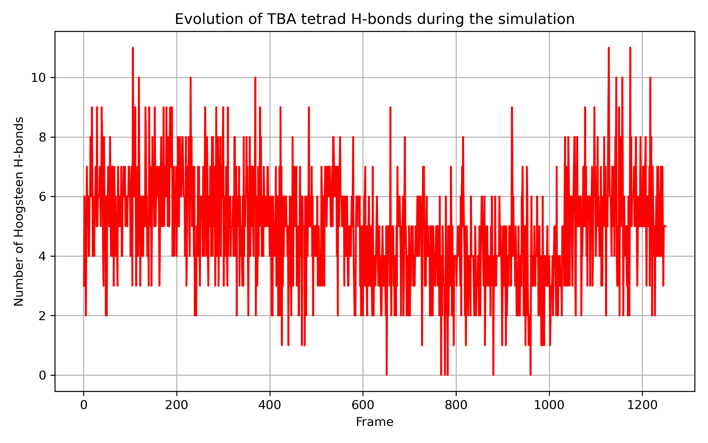
Number of Hoogsteen hydrogen bonds in the tetrads

The obtained results clearly show that the average number of hydrogen bonds decreases by approximately two when the structure partially opens between frames 400 and 1000.