ORCA

Introduction

ORCA is a general-purpose quantum chemistry software package that supports a wide range of electronic structure calculations, from simple semi-empirical methods and modern DFT approaches to highly accurate coupled-cluster methods. It is particularly well suited for the investigation of molecular geometries, reaction mechanisms, spectroscopic properties, and thermodynamic parameters.

The purpose of this documentation is to introduce the most important applications of ORCA through practical examples. Each chapter can be followed independently; however, it is recommended to work through the examples in the order presented, since later calculations often build upon concepts and procedures introduced earlier.

Structure of an ORCA Input File

ORCA calculations are controlled through simple text-based input files, which typically use the .inp file extension.

A minimal ORCA input file consists of three main parts:

specification of the calculation type,
molecular charge and multiplicity,
atomic coordinates.

Example: simple energy calculation for a water molecule

! B3LYP def2-SVP

* xyz 0 1
O    0.000000    0.000000    0.000000
H    0.758602    0.000000    0.504284
H   -0.758602    0.000000    0.504284
*

Components of the Input File

Method and Basis Set

The first line contains the most important calculation parameters.

! B3LYP def2-SVP

In this example:

B3LYP is the selected density functional.

A list of available DFT functionals can be found at:

https://orca-manual.mpi-muelheim.mpg.de/contents/modelchemistries/DensityFunctionalTheory.html

def2-SVP is the basis set used.

Available basis sets can be found at:

https://orca-manual.mpi-muelheim.mpg.de/contents/essentialelements/basisset.html

Multiple keywords can be specified on the same line after the exclamation mark.

Charge and Multiplicity

* xyz 0 1

The first number corresponds to the total charge of the system, while the second number specifies the multiplicity.

For a water molecule, the charge is 0 and the multiplicity is 1, corresponding to a neutral closed-shell system.

Atomic Coordinates

Coordinates are specified in units of Angstroms. Each line describes one atom.

O    0.000000    0.000000    0.000000

The format is:

AtomName     X     Y     Z

The coordinate block is terminated by a standalone * character.

Input File Naming Convention

Throughout the examples in this documentation, the following naming convention will be used:

water.inp
ethanol_opt.inp
benzene_tddft.inp
methane_nmr.inp

This naming scheme makes it easier to identify the results associated with each calculation. In the next chapter, we will discuss how to run ORCA calculations and describe the most important components of the generated output files, which will be used throughout the examples presented later in this documentation.

Running ORCA

ORCA calculations can be launched from the command line. Based on the input file, the program automatically performs the requested quantum chemical calculation and generates several output files.

Starting a Calculation

Assume that we have created the following input file:

water.inp

The calculation can then be executed as follows:

orca water.inp > water.out

Components of the command:

orca: the ORCA executable
water.inp: the input file
>: redirects terminal output to a file
water.out: the output file of the calculation, containing detailed results and diagnostic information (the information is written to this file instead of being displayed on the screen)

Verifying Successful Completion

After the calculation has finished, it is always advisable to inspect the end of the output file.

tail -n 20 water.out

For a successful calculation, the following line should appear:

****ORCA TERMINATED NORMALLY****

This indicates that the calculation completed without errors.

Output Files

After a simple geometry optimization, the following files may be generated:

water.inp
water.out
water.gbw
water.xyz
water.opt.xyz
water_property.txt

The exact set of generated files depends on the type of calculation being performed.

water.out
The most important output file. It contains:
calculation parameters,

SCF cycles,

energies,

geometry optimization steps,

final results.
Most information required for analysis can be obtained from this file.
water.gbw
ORCA’s binary wavefunction file. It contains, among other things:
molecular orbitals,

electron density information,

wavefunction data.
Subsequent calculations often use this file as a starting point.
water.xyz

An XYZ file containing the coordinates currently used during the calculation. It is primarily useful for inspection and visualization.
water.opt.xyz
For geometry optimizations, this file contains the final optimized structure. It is one of the most frequently used output files.

The file can be opened directly in programs such as:
ChimeraX

Avogadro

IQmol

VMD
for visualization and further analysis.

Finding the Most Important Results

Total Energy

The final energy can be found in the output file by searching for the following line:

FINAL SINGLE POINT ENERGY

For example:

FINAL SINGLE POINT ENERGY     -76.27268654

The energy is reported in atomic units (Hartree).

Optimization Convergence

For geometry optimization calculations, look for the following message:

THE OPTIMIZATION HAS CONVERGED

This indicates that ORCA has successfully located a local minimum on the potential energy surface.

SCF Convergence

Successful convergence of the electronic structure calculation is indicated by the following line:

SCF HAS CONVERGED AFTER

For example:

SCF HAS CONVERGED AFTER 10 CYCLES

If the SCF procedure does not converge, the subsequent results cannot be considered reliable.

Importance of Output Files for Subsequent Calculations

Throughout the remainder of this documentation, we will primarily make use of the following output files:

.out: energies, spectroscopic data, and convergence information;
.gbw: wavefunction files that can be reused in subsequent calculations;
.opt.xyz: optimized geometries for frequency calculations, TD-DFT, NMR studies, or higher-level energy calculations.

In the next chapter, we present the first practical example of this documentation: the geometry optimization of a water molecule, explained step by step.

Example 1 - Geometry Optimization of a Water Molecule

In this example, we perform a geometry optimization of a water molecule (H₂O). The aim is to demonstrate how the most stable structure of a molecule can be determined using a quantum chemical method.

Geometry optimization is one of the most frequently used ORCA calculations, since almost all subsequent studies (frequency calculations, TDDFT, NMR, reaction energy calculations, etc.) require an optimized geometry.

Creating the Input File

Create the file water_opt.inp, containing:

! B3LYP def2-SVP Opt

* xyz 0 1
O    0.000000    0.200000    0.000000
H    1.200000    0.000000    0.000000
H   -1.200000    0.000000    0.000000
*

Calculation parameters:

B3LYP: the selected hybrid DFT functional
def2-SVP: the selected medium-sized basis set
Opt: perform geometry optimization

The coordinates define the initial molecular structure.

Running the Calculation

Start the calculation from the command line:

nohup $(which orca) water_opt.inp > water_opt.out 2>&1 &

Components of the command:

nohup: ensures that the calculation continues even if the user logs out of the server
$(which orca): finds the full path of the ORCA executable currently in use
water_opt.inp: the ORCA input file
> water_opt.out: redirects the standard output of ORCA to the specified output file
2>&1: redirects error messages to the same output file
&: launches the calculation as a background process, immediately returning control to the terminal

Monitoring the Calculation

The progress of the calculation can be monitored continuously:

tail -f water_opt.out

This command continuously displays newly appended lines from the output file.

Checking the Calculation

Near the end of the output file (water_opt.out), look for the following line:

THE OPTIMIZATION HAS CONVERGED

This indicates that the geometry optimization has completed successfully.

At the very end of the file, the following message should also appear:

****ORCA TERMINATED NORMALLY****

indicating that the calculation finished without errors.

Optimized Structure

The final optimized structure can be found in:

water_opt.xyz

The geometry optimization trajectory is stored in:

water_opt_trj.xyz

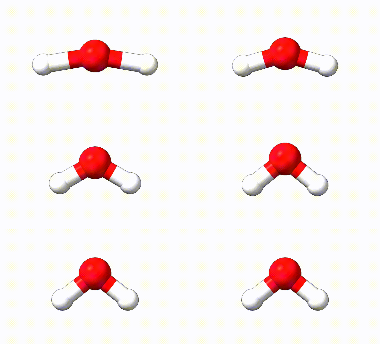
../_images/water_opt.gif — Geometry optimization of a water molecule.

It can be clearly seen that the atomic coordinates change relative to the initial geometry as the optimization proceeds.

Extracting the Energy

In the output file, locate the following line:

FINAL SINGLE POINT ENERGY

For example:

FINAL SINGLE POINT ENERGY       -76.187498531589

This is the electronic energy of the optimized structure expressed in Hartree units.

In the next chapter, we will perform a frequency calculation on an optimized ethanol molecule, from which thermochemical properties and an IR spectrum can be obtained.

Example 2 - Frequency Calculation and Thermochemistry of Ethanol

Frequency calculations are one of the most important steps in a quantum chemistry workflow.

They can be used to determine:

vibrational spectrum
IR spectrum
zero-point energy (ZPE)
entropy
enthalpy
Gibbs free energy

Starting Structure

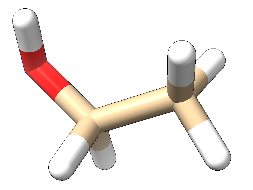
Frequency calculations should always be performed on an optimized geometry. In this example, we use a previously optimized ethanol structure (ethanol_opt.xyz).

Input File (ethanol_freq.inp)

! B3LYP def2-SVP Freq

* xyzfile 0 1 ethanol_opt.xyz

The input file simply reads the structure obtained from the previous geometry optimization.

Running the Calculation

nohup $(which orca) ethanol_freq.inp > ethanol_freq.out 2>&1 &

Examining the Vibrational Frequencies

In the output file (ethanol_freq.out), locate the following section:

VIBRATIONAL FREQUENCIES

This section contains the normal vibrational modes of the molecule.

Verification of a Minimum

An optimized structure can only be considered a true minimum if all vibrational frequencies are positive.

For example:

      0.00 cm**-1
      0.00 cm**-1
      0.00 cm**-1
      0.00 cm**-1
      0.00 cm**-1
      0.00 cm**-1
    274.70 cm**-1
    314.01 cm**-1
    424.92 cm**-1

If all frequencies are positive, the geometry optimization was successful. If a negative (imaginary) frequency appears, the structure corresponds to a saddle point rather than a minimum.

Thermochemical Data

Near the end of the output file, the following section can be found:

THERMOCHEMISTRY AT 298.15 K

This block contains:

ZPE
enthalpy
entropy
Gibbs free energy

IR Spectrum

ORCA also calculates IR intensities for each vibrational mode.

For example:

-----------
IR SPECTRUM
-----------

Mode   freq       eps      Int      T**2         TX        TY        TZ
    cm**-1   L/(mol*cm) km/mol    a.u.
----------------------------------------------------------------------------
6:    274.70   0.000956    4.83  0.001085  ( 0.011723  0.026853  0.015065)
7:    314.01   0.022173  112.05  0.022035  (-0.095752 -0.075734 -0.084448)
8:    424.92   0.003954   19.98  0.002904  (-0.029891 -0.038557 -0.022879)
9:    804.98   0.000545    2.75  0.000211  (-0.003175  0.008365  0.011456)
10:   895.42   0.001430    7.23  0.000498  (-0.017717  0.013081  0.003640)

A theoretical IR spectrum can be generated directly from these data.

In the next example, we will calculate the UV-Vis spectrum of caffeine using the TDDFT method.

Example 3: UV-Vis Spectrum Calculation of Caffeine Using TDDFT

After geometry optimization and frequency calculations, one of the most common applications is the investigation of the electronic excited states of molecules. Using Time-Dependent Density Functional Theory (TDDFT), ORCA can determine:

the energies of electronic transitions,
absorption wavelengths,
oscillator strengths,
the data required to generate a UV-Vis spectrum.

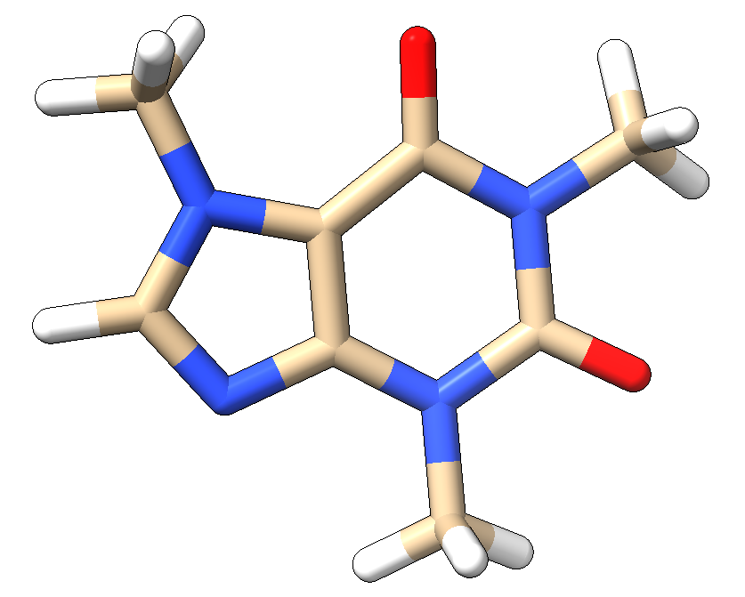
In this example, we calculate the UV-Vis spectrum of caffeine.

Starting Structure

TDDFT calculations should generally be performed on a previously optimized geometry. Let us assume that the file caffeine_opt.xyz is available.

Creating the Input File

Create the file caffeine_tddft.inp with the following contents:

! B3LYP def2-TZVP TightSCF

%tddft
   nroots 10
end

* xyzfile 0 1 caffeine_opt.xyz

Calculation parameters:

B3LYP: hybrid DFT functional used for the excited-state calculation;
def2-TZVP: basis set employed in the calculation;
TightSCF: stricter SCF convergence criterion;
nroots 10: requests the first 10 excited states.

Running the Calculation

nohup $(which orca) caffeine_tddft.inp > caffeine_tddft.out 2>&1 &

Analysis of the Excited States

The results can be found in the output file caffeine_tddft.out.

Search for the following section:

ABSORPTION SPECTRUM VIA TRANSITION ELECTRIC DIPOLE MOMENTS

In this block, ORCA lists the individual electronic transitions. For example:

----------------------------------------------------------------------------------------------------
    Transition      Energy     Energy  Wavelength fosc(D2)      D2        DX        DY        DZ
                    (eV)      (cm-1)    (nm)                 (au**2)    (au)      (au)      (au)
----------------------------------------------------------------------------------------------------
0-1A  ->  1-1A    4.832128   38973.7   256.6   0.162204719   1.37015   0.50550   1.05570   0.01118
0-1A  ->  2-1A    4.973880   40117.0   249.3   0.000094667   0.00078   0.00079  -0.00262   0.02774
0-1A  ->  3-1A    5.714423   46089.9   217.0   0.017515644   0.12511  -0.27151   0.22431   0.03283
0-1A  ->  4-1A    5.997017   48369.2   206.7   0.000240572   0.00164  -0.00018  -0.00002   0.04046
0-1A  ->  5-1A    6.087781   49101.3   203.7   0.006869797   0.04606  -0.03328   0.01491  -0.21150
0-1A  ->  6-1A    6.104293   49234.4   203.1   0.140840946   0.94175  -0.92552   0.27654   0.09318
0-1A  ->  7-1A    6.166793   49738.5   201.1   0.000012226   0.00008   0.00193   0.00007  -0.00879
0-1A  ->  8-1A    6.256579   50462.7   198.2   0.000033049   0.00022  -0.00283  -0.00834  -0.01175
0-1A  ->  9-1A    6.287600   50712.9   197.2   0.050501324   0.32784   0.17656   0.54452   0.01283
0-1A  -> 10-1A    6.487421   52324.6   191.1   0.521479505   3.28101  -1.80479  -0.02401   0.15219

Meaning of the columns:

Energy (eV): transition energy in electronvolts;
Energy (cm⁻¹): transition energy expressed as a wavenumber;
Wavelength (nm): wavelength corresponding to the transition;
fosc(D2): oscillator strength of the transition.

The larger the fosc(D2) value, the more intense the corresponding absorption band is expected to be in the experimental UV-Vis spectrum.

Plotting the Spectrum

The TDDFT results can be exported to a spreadsheet or plotting software. For example, the following data should be collected:

λ (nm)	fosc
256.6	0.16220
249.3	0.00009
217.0	0.01752
206.7	0.00024
203.7	0.00687
203.1	0.14084
201.1	0.00001
198.2	0.00003
197.2	0.05050
191.1	0.52148

A simulated UV-Vis spectrum can be generated by applying Gaussian broadening functions to the transitions using the corresponding oscillator strengths and wavelengths.

The spectrum can be plotted using, for example:

Microsoft Excel,
Origin,
Python,
SpectraGryph.

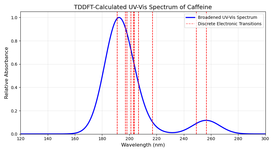
Python script used to create the plot:

UV_Vis_spec_plot.py

Limitations of TDDFT Calculations

The calculated absorption maxima generally do not exactly match the experimental values.

The most common sources of deviation are:

limitations of the selected density functional,
the size of the basis set,
neglect of solvent effects,
the absence of vibronic coupling effects.

Therefore, TDDFT results are primarily suitable for qualitative or semi-quantitative comparisons.

Outlook: Higher-Accuracy UV-Vis Spectra Using the CASSCF Method

The TDDFT method provides fast and generally reliable results for most organic molecules. However, it may encounter limitations for certain systems, particularly:

strongly correlated electronic systems,
transition-metal complexes,
molecules containing nearly degenerate orbitals,
systems involving multi-electron excitations.

In such cases, a more accurate description can be achieved using multireference methods such as CASSCF (Complete Active Space Self-Consistent Field) calculations.

In the CASSCF approach, the user defines an active space that contains the molecular orbitals and electrons most relevant to the electronic transitions under investigation. ORCA then performs a full configuration interaction within this active space, which can significantly improve the description of excited states.

In practice, the following workflow is typically employed:

Geometry optimization
Generation of molecular orbitals or Natural Orbitals
Definition of the active space
Execution of a CASSCF calculation
Optional application of a NEVPT2 correction
Generation of a UV-Vis spectrum from the excited states

Example 4 - Calculation of NMR Chemical Shifts for Methane

Following geometry optimization, frequency calculations, and UV-Vis spectroscopic applications, one of the most important applications of quantum chemical calculations is the determination of NMR parameters.

ORCA can calculate:

magnetic shielding tensors,
isotropic shielding constants,
chemical shifts,
spin-spin coupling constants.

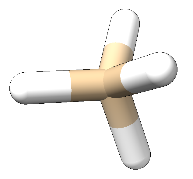
In NMR spectroscopy, the most commonly studied nuclei are ¹H (hydrogen-1) and ¹³C (carbon-13). These isotopes possess nuclear spin, making them NMR-active and experimentally observable.

Starting Structure

NMR calculations are generally performed on previously optimized geometries. Assume that the file methane_opt.xyz is available.

Creating the Input File

We create the file methane_nmr.inp with the following contents:

! B3LYP def2-TZVP NMR TightSCF

* xyzfile 0 1 methane_opt.xyz

Calculation parameters:

B3LYP: the selected hybrid DFT functional
def2-TZVP: a triple-zeta quality basis set
TightSCF: stricter SCF convergence criteria
NMR: calculation of NMR shielding constants

Running the Calculation

nohup $(which orca) methane_nmr.inp > methane_nmr.out 2>&1 &

Locating the NMR Results

In the output file (methane_nmr.out), search for the following section:

CHEMICAL SHIELDING SUMMARY (ppm)

This section contains the calculated shielding constants for each atom. For example:

 Nucleus  Element    Isotropic     Anisotropy
-------  -------  ------------   ------------
     H           31.359          8.679
     C          187.825          0.019
     H           31.358          8.680
     H           31.358          8.679
     H           31.358          8.679

Interpretation of the results:

Nucleus: atom index within the molecule
Element: chemical symbol of the atom
Isotropic: isotropic shielding constant (σ), used to calculate NMR chemical shifts
Anisotropy: anisotropy of the shielding tensor, indicating how strongly the magnetic environment of the nucleus depends on direction

Based on the results shown above, the four hydrogen atoms possess virtually identical isotropic shielding constants, which is fully consistent with the tetrahedral symmetry of methane.

Calculation of Chemical Shifts

ORCA directly calculates the shielding constant:

\[\sigma\]

To determine the chemical shift, a reference compound is required. For organic molecules, the most commonly used reference is TMS (tetramethylsilane). The chemical shift is defined as:

\[\delta = \sigma_{ref} - \sigma\]

where

$\sigma_{ref}$ is the shielding constant of TMS,
$\sigma$ is the shielding constant of the atom under investigation.

For methane, the following isotropic shielding constants were obtained:

13C : 187.825 ppm
1H : 31.359 ppm

The results of the TMS reference calculation are:

13C : 181.459 ppm
1H : 31.579 ppm

The resulting chemical shifts are:

\[\delta (^{13}C) = 181.459 - 187.825 = -6.37~ppm\]

\[\delta (^{1}H) = 31.579 - 31.359 = 0.22~ppm\]

It can be seen that the carbon atom in methane is more strongly shielded than in TMS and therefore exhibits a negative ¹³C chemical shift. For the protons, the calculated value of 0.22 ppm is in good agreement with the expected experimental ¹H NMR signal of methane.

This example illustrates how the shielding constants calculated directly by ORCA can be converted into the chemical shifts commonly reported in experimental NMR spectra.

In the next chapter, we demonstrate transition-state (TS) searching with ORCA through the investigation of a simple reaction mechanism.

Example 5 - Transition State Search for an SN2 Reaction

One of the most important applications of quantum chemical calculations is the investigation of reaction mechanisms. The rate and course of a reaction are fundamentally determined by the transition state (TS), which corresponds to the top of the energy barrier separating reactants and products.

In this example, we search for the transition state of a classical SN2 reaction:

\[\mathrm{Cl^- + CH_3Br \rightarrow CH_3Cl + Br^-}\]

The SN2 reaction is an ideal teaching example because its mechanism is well understood and the transition state can be identified unambiguously.

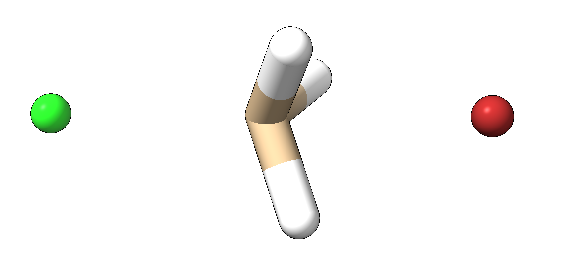
The Concept of a Transition State

During the reaction, the nucleophilic chloride ion approaches the carbon atom from one side while the bromine atom leaves from the opposite side.

In the transition state:

the C-Cl bond is not yet fully formed,
the C-Br bond is not yet completely broken.

The transition state corresponds to the highest-energy point along the entire reaction pathway.

Creating the Input File

Assume that an initial transition-state guess is available in the file: sn2_ts_guess.xyz

Create the input file sn2_ts.inp with the following contents:

! B3LYP def2-TZVP OptTS TightSCF

* xyzfile -1 1 sn2_ts_guess.xyz

Calculation parameters:

OptTS: transition-state optimization;
B3LYP: selected hybrid DFT functional;
def2-TZVP: triple-zeta quality basis set;
TightSCF: stricter SCF convergence criteria.

Running the Calculation

nohup $(which orca) sn2_ts.inp > sn2_ts.out 2>&1 &

After confirming successful optimization by locating the message

THE GEOMETRY HAS CONVERGED

the resulting structure can be examined in the file sn2_ts.xyz.

Verification of the Transition State

Optimization alone does not prove that a true transition state has been found. To verify this, a frequency calculation must be performed. A detailed description of this procedure can be found in Section Example 2 - Frequency Calculation and Thermochemistry of Ethanol.

In the output file sn2_ts_freq.out, search for the section:

VIBRATIONAL FREQUENCIES

For a genuine transition state, exactly one imaginary (negative) frequency must be present. In our example:

      0.00 cm**-1
      0.00 cm**-1
      0.00 cm**-1
      0.00 cm**-1
      0.00 cm**-1
      0.00 cm**-1
   -304.06 cm**-1  ***imaginary mode***
    169.18 cm**-1
    172.36 cm**-1
    172.39 cm**-1
    865.46 cm**-1
    865.59 cm**-1
    995.53 cm**-1
   1408.52 cm**-1
   1408.63 cm**-1
   3200.27 cm**-1
   3391.17 cm**-1
   3391.34 cm**-1

Here, the frequency of -304.06 cm^-1 corresponds to the vibrational mode associated with the reaction coordinate.

Interpretation of the Results

The following rules apply when evaluating a transition state:

0 negative frequencies → minimum structure
1 negative frequency → transition state
2 or more negative frequencies → higher-order saddle point

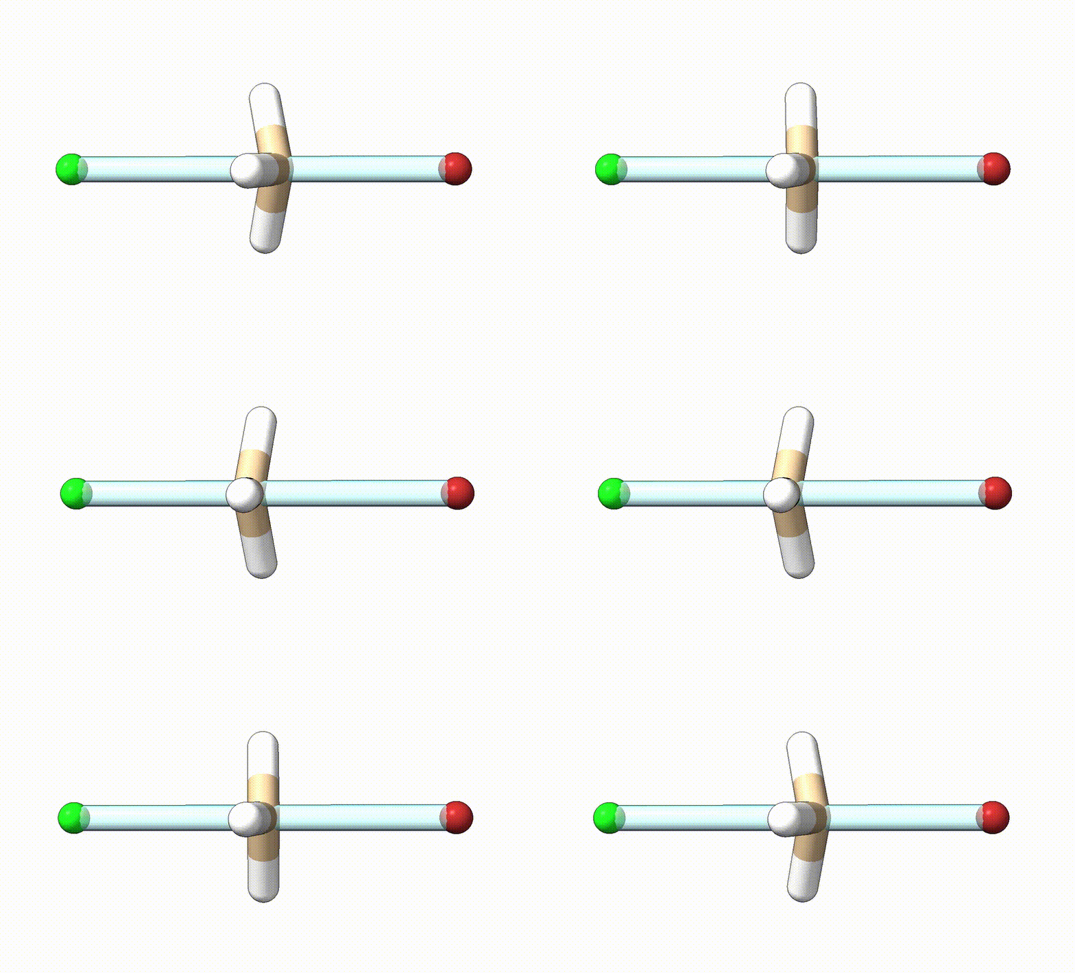
By animating the vibrational mode associated with the imaginary frequency, it can be verified whether the reaction coordinate indeed corresponds to the breaking of the C-Br bond and the formation of the C-Cl bond.

Visualization in ChimeraX

ChimeraX is capable of reading ORCA .out files. If the file sn2_ts_freq.out is opened, the vibrational mode associated with the imaginary frequency can be displayed.

Tools → Quantum Chemistry → Visualize Normal Modes

Activation Energy

By comparing the energy of the transition state with that of the reactant, the activation energy can be determined:

\[E_a = E_{TS} - E_{reactant}\]

This quantity is directly related to the reaction rate.

Example 6 - Including Solvent Effects in ORCA

A significant portion of quantum chemical calculations focuses on processes that occur in solution. The presence of a solvent can have a substantial impact on:

molecular stability,
reaction energies,
geometric parameters,
UV-Vis spectra,
NMR chemical shifts.

ORCA supports several implicit solvent models, the most commonly used being:

CPCM (Conductor-like Polarizable Continuum Model)
SMD

In this example, we demonstrate the geometry optimization of a caffeine molecule in aqueous solution.

Optimization in Aqueous Solution Using the CPCM Model

Input file (caffeine_opt_cpcm_wat.inp):

! B3LYP def2-TZVP Opt TightSCF CPCM(Water)

%pal
  nprocs 40
end

* xyz 0 1
N      1.5808      0.7027     -0.2279
C      1.7062     -0.7374     -0.2126
N      0.5340     -1.5671     -0.3503
C      0.3231      1.3600      0.0274
C     -0.8123      0.4553      0.0817
C     -0.6967     -0.9322     -0.0662
N     -2.1886      0.6990      0.2783
C     -2.8512     -0.5205      0.2532
N     -1.9537     -1.5188      0.0426
C      0.6568     -3.0274     -0.1675
O      2.8136     -1.2558     -0.1693
O      0.2849      2.5744      0.1591
C     -2.8096      2.0031      0.5032
C      2.8301      1.5004     -0.1968
H     -3.9271     -0.6787      0.3762
H      1.4823     -3.4046     -0.7865
H     -0.2708     -3.5204     -0.4868
H      0.8567     -3.2990      0.8788
H     -2.4123      2.7478     -0.2017
H     -2.6042      2.3621      1.5221
H     -3.8973      1.9344      0.3695
H      3.5959      1.0333     -0.8314
H      3.2249      1.5791      0.8255
H      2.6431      2.5130     -0.5793
*

In this example, the most important keyword is CPCM(Water), which models the molecule in aqueous solution using the CPCM continuum solvation model.

Running the Calculation

nohup $(which orca) caffeine_opt_cpcm_wat.inp > caffeine_opt_cpcm_wat.out 2>&1 &

The calculation produces the optimized geometry caffeine_opt_cpcm_wat.xyz and the output file caffeine_opt_cpcm_wat.out.

Optimization in Aqueous Solution Using the SMD Model

The SMD model generally provides more accurate results. The input file (caffeine_opt_smd_wat.inp) is:

! B3LYP def2-TZVP Opt TightSCF CPCM

%cpcm
  smd true
  SMDsolvent "Water"
end

%pal
  nprocs 40
end

* xyz 0 1
N      1.5808      0.7027     -0.2279
C      1.7062     -0.7374     -0.2126
N      0.5340     -1.5671     -0.3503
C      0.3231      1.3600      0.0274
C     -0.8123      0.4553      0.0817
C     -0.6967     -0.9322     -0.0662
N     -2.1886      0.6990      0.2783
C     -2.8512     -0.5205      0.2532
N     -1.9537     -1.5188      0.0426
C      0.6568     -3.0274     -0.1675
O      2.8136     -1.2558     -0.1693
O      0.2849      2.5744      0.1591
C     -2.8096      2.0031      0.5032
C      2.8301      1.5004     -0.1968
H     -3.9271     -0.6787      0.3762
H      1.4823     -3.4046     -0.7865
H     -0.2708     -3.5204     -0.4868
H      0.8567     -3.2990      0.8788
H     -2.4123      2.7478     -0.2017
H     -2.6042      2.3621      1.5221
H     -3.8973      1.9344      0.3695
H      3.5959      1.0333     -0.8314
H      3.2249      1.5791      0.8255
H      2.6431      2.5130     -0.5793
*

Important Keywords in the Input File

B3LYP: selected DFT functional;
def2-TZVP: basis set used in the calculation;
Opt: requests a geometry optimization;
TightSCF: applies stricter SCF convergence criteria;
CPCM: activates the continuum solvation model, placing the molecule in a cavity surrounded by solvent and providing the framework required for SMD solvation calculations.

Components of the %cpcm block:

smd true: activates the SMD solvation model and accounts not only for electrostatic interactions but also for non-electrostatic solvent effects;
SMDsolvent "Water": specifies the solvent used in the calculation (in this example, liquid water).

Running the Calculation

nohup $(which orca) caffeine_opt_smd_wat.inp > caffeine_opt_smd_wat.out 2>&1 &

The calculation produces the optimized geometry caffeine_opt_smd_wat.xyz and the corresponding output file caffeine_opt_smd_wat.out.

Investigation of Solvation Effects

The energies obtained from gas-phase and solvent-phase calculations can be compared. For example, based on the

FINAL SINGLE POINT ENERGY

lines:

System	Energy (Eh)
Gas phase	-680.262346702581
Water (CPCM)	-680.281556102020
Water (SMD)	-680.282052379311

The decrease in energy reflects the stabilizing effect of the solvent.

RMSD Values Between the Different Geometries

The values were determined using ChimeraX.

Systems	RMSD (Å)
Gas phase-CPCM	0.014
Gas phase-SMD	0.021
CPCM-SMD	0.015

These low RMSD values indicate that the application of implicit solvent models only slightly modifies the equilibrium geometry of caffeine.

Example 7 - High-Accuracy Energy Calculation Using DLPNO-CCSD(T)

In the previous sections of this documentation, we primarily used DFT-based methods. DFT methods generally provide a good balance between computational cost and accuracy; however, in certain situations, more accurate energy values may be required.

One of ORCA’s greatest strengths is its support for the DLPNO-CCSD(T) method, which is based on an approximation of the CCSD(T) approach, often referred to as the “gold standard” of quantum chemistry. The DLPNO (Domain-Based Local Pair Natural Orbital) approximation dramatically reduces computational cost while retaining most of the accuracy of the parent method.

What Can DLPNO-CCSD(T) Be Used For?

The method is commonly applied to:

calculation of reaction energies;
refinement of activation energies;
calculation of binding energies;
validation of DFT results;
generation of publication-quality energy values.

A typical workflow is:

geometry optimization using a DFT method;
frequency calculation;
single-point energy calculation at the DLPNO-CCSD(T) level.

Geometry optimizations at the CCSD(T) level are extremely computationally expensive. Therefore, in practice, DLPNO-CCSD(T) single-point energy calculations are almost always performed on geometries optimized using DFT. This approach allows the geometry to be determined efficiently while providing final energies that are significantly more accurate than those obtained from a purely DFT-based calculation.

Creating the Input File

Assume that an optimized water geometry at the B3LYP/def2-TZVP level is already available: water_opt.xyz

Create the file water_dlpnoccsdt.inp with the following contents:

! DLPNO-CCSD(T) def2-TZVP TightSCF TightPNO AutoAux

* xyzfile 0 1 water_opt.xyz

Calculation parameters:

DLPNO-CCSD(T): the electronic structure method
def2-TZVP: a triple-zeta quality basis set
TightSCF: stricter SCF convergence criteria
TightPNO: stricter DLPNO thresholds, which generally yield more accurate energies
AutoAux: automatically generates the auxiliary basis sets required for DLPNO calculations

Running the Calculation

nohup $(which orca) water_dlpnoccsdt.inp > water_dlpnoccsdt.out 2>&1 &

Determination of the Final Energy

In the output file water_dlpnoccsdt.out, search for the following line near the end of the file:

FINAL SINGLE POINT ENERGY

In this example:

FINAL SINGLE POINT ENERGY       -76.326498113918

This is the electronic energy calculated at the DLPNO-CCSD(T) level of theory.

Let us assume that a previous B3LYP calculation was performed on the same structure, yielding:

FINAL SINGLE POINT ENERGY       -76.426048175333

The two energies cannot be compared directly between different molecules. However, for different conformers, reaction states, or structures of the same system, the energy differences provide highly valuable information.

Limitations of DLPNO-CCSD(T)

Although the method is significantly faster than conventional CCSD(T), it is still substantially more computationally demanding than a typical DFT calculation. Therefore, DLPNO-CCSD(T) calculations are usually employed for:

optimized geometries,
final energy refinement,
a limited number of molecular structures.

Most Commonly Used ORCA Keywords

Opt: geometry optimization to locate a local minimum;
Freq: calculation of vibrational frequencies, IR spectra, and thermochemical properties;
OptTS: transition-state optimization;
ScanTS: relaxed coordinate scan and automatic transition-state search;
TDDFT: calculation of excited states and UV-Vis spectra;
NMR: calculation of shielding constants and NMR parameters;
DLPNO-CCSD(T): highly accurate correlation energy calculation;
TightSCF: stricter SCF convergence criteria;
SlowConv: recommended for systems with difficult SCF convergence;
VeryTightSCF: exceptionally strict SCF convergence settings.

Basis Sets

def2-SVP: medium-sized double-zeta basis set;
def2-TZVP: triple-zeta quality general-purpose basis set;
def2-TZVPP: triple-zeta basis set with additional polarization functions;
def2-QZVP: high-accuracy quadruple-zeta basis set.

Popular DFT Functionals

B3LYP: the most widely used hybrid functional;
PBE0: a generally reliable hybrid functional;
wB97X-D4: a modern range-separated functional including dispersion corrections;
r2SCAN-3c: a fast and cost-effective method for geometry optimization and large systems.

Dispersion Corrections

D3: Grimme’s D3 dispersion correction with Becke-Johnson damping;
D4: modern dispersion correction scheme.

Solvent Models

CPCM: continuum solvation model;
SMD: more advanced solvation model.

Parallel Execution and Memory Usage

ORCA can efficiently take advantage of multi-core processors. Therefore, for larger calculations it is advisable to specify both the number of processor cores available and the amount of memory that can be used.

Specifying the Number of Processor Cores

Parallelization can be configured using the %pal block.

For example, to use 8 processor cores:

%pal
   nprocs 8
end

The complete input file would then look like:

! B3LYP def2-TZVP Opt

%pal
   nprocs 8
end

* xyzfile 0 1 molecule.xyz

In this case, ORCA will use eight CPU cores during the calculation.

Memory Settings

The amount of memory available for the calculation can be specified using the %maxcore keyword.

For example:

%maxcore 4000

This means that ORCA may use approximately 4000 MB of memory per CPU core.

The total memory requirement is therefore:

\[N_{\mathrm{cores}} \times MaxCore\]